10 t-Tests and Their Rank-Based Alternatives
Parametric test of mean differences. It is used when:
- The criterion/dependent variable (DV) is measured on an interval or ratio scale;
- The mean of one group is compared with a known or hypothesized value (one-sample t-Test);
- The means of two groups are compared. There is a single predictor/independent variable (IV), measured on a nominal scale, that can have only two values (independent samples t-Test);
- Two measurements that are related in some way are compared, such as the same participants measured before and after a treatment (paired samples t-Test).
When the DV is ordinal, or when it is clearly not normally distributed in a small sample, each of the three tests has a rank-based alternative11 Rank-based tests are also called non-parametric tests, because they do not assume that the data follows a particular distribution, such as the normal distribution.. Each alternative answers a closely related question, about ranks or medians rather than means, and is described right after its t-Test, on the same data. Table 10.1 shows which test to use.
1 Rank-based tests are also called non-parametric tests, because they do not assume that the data follows a particular distribution, such as the normal distribution.
| Design | Normal data | Ordinal or not normal | Direction or median only |
|---|---|---|---|
| One group against a known value | One-sample t-Test | One-sample Wilcoxon | Sign test |
| Two independent groups | Independent samples t-Test | Mann-Whitney U | Mood’s median test |
| Two related measurements | Paired samples t-Test | Wilcoxon signed-rank | Sign test |
The design of the study picks the row, and the data picks the column. Normal data means a DV measured on an interval or ratio scale and normally distributed. The tests further to the right make fewer assumptions, but they use less of the information in the data and, when the data is normal, have less power to detect a difference22 With heavy tails or outliers, the rank-based tests can have more power than the t-Tests.. They also compare something slightly different: ranks or medians, not means. The test furthest to the left whose assumptions are met is therefore the one to use. When the standard deviation of the population is known, the one-sample z test replaces the one-sample t-Test. More than two groups are compared with the ANOVA, and more than two measurements with the repeated-measures ANOVA. When the DV has only two categories, such as Yes and No, two related measurements are compared with McNemar’s test.
2 With heavy tails or outliers, the rank-based tests can have more power than the t-Tests.
The t-Test is easier to understand once we know where it comes from. The chapter therefore starts with its simpler predecessor, the z test, and with the idea both tests are built on, the sampling distribution.
10.1 The One-Sample z Test
At a glance
- Question
- Does the mean of a sample differ from a known population mean?
- Design
- One group, one measurement, compared with a population whose standard deviation is known
- Dependent variable
- Interval or ratio
- Assumptions
-
- Independent observations: each participant is measured once
- Randomly selected sample
- DV normally distributed, or a sample large enough for the central limit theorem
- The standard deviation of the population is known
- Null hypothesis
- The mean of the population the sample comes from equals the known mean (\mu = \mu_{0})
- Test statistic
- z
- Effect size
- Cohen’s d: 0.2 small, 0.5 medium, 0.8 large
- If conditions fail
-
- The standard deviation of the population is not known → One-sample t-Test
- Include in the write-up
-
- The sample size, mean, and standard deviation, and the population mean and standard deviation
- z = …, p = …
- Cohen’s d
Used when the mean of a sample is compared with the mean of a population whose standard deviation is known33 This is rarely the case in practice, but it does happen. Standardized tests, for example, publish the mean and the standard deviation of the population they were normed on, usually a large, representative sample of the people the test is meant for.. The question the z test answers is: Is my sample different from the population it is compared with?
3 This is rarely the case in practice, but it does happen. Standardized tests, for example, publish the mean and the standard deviation of the population they were normed on, usually a large, representative sample of the people the test is meant for.
10.1.1 The Sampling Distribution
Imagine drawing a sample of 36 people from a population and computing their mean. A second sample of 36 people would have a slightly different mean, and so would a third. If we could draw all possible samples of the same size and compute the mean of each one, the means would form a distribution of their own, the sampling distribution of the mean. Most sample means would fall close to the population mean, and only a few, by chance, far from it.
We cannot draw all possible samples, but we can simulate many of them. Let’s take a population with a mean of \mu = 70 and a standard deviation of \sigma = 12, draw 10,000 samples of 36 values from it, and keep the mean of each sample.
[1] 70.00441[1] 2.02063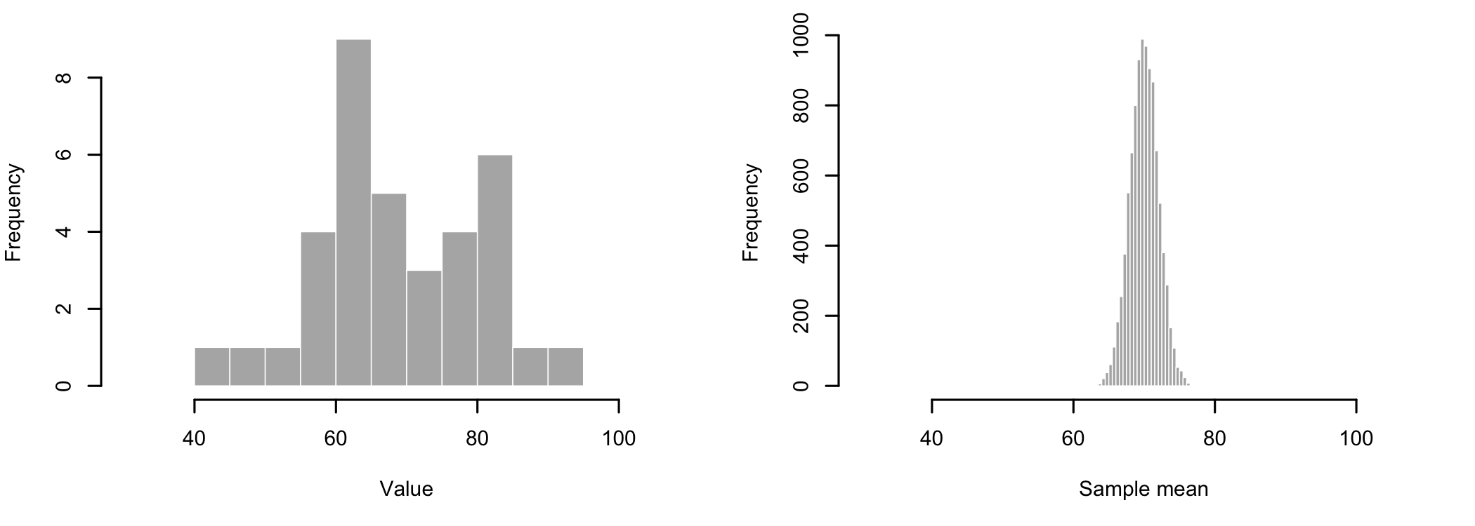
Figure 10.1 shows the difference between the values in one sample (left) and the means of many samples (right). The sample means are grouped much more tightly around the population mean than the individual values. Their mean, 70.00, is almost exactly the population mean, and their standard deviation, 2.02, is much smaller than the standard deviation of the population. The standard deviation of the sampling distribution is called the standard error of the mean (\sigma_{\bar{x}}), and it does not need a simulation to be found:
\sigma_{\bar{x}} = \frac{\sigma}{\sqrt{n}} = \frac{12}{\sqrt{36}} = 2
The central limit theorem adds that the sampling distribution of the mean is approximately normal for samples that are large enough, often taken as about 30 or more, even when the population itself is not normally distributed44 How large is large enough depends on the population. A strongly skewed population, or one with outliers, may need many more.. These two facts allow us to tell how unusual a sample mean is, by placing it on the sampling distribution55 A sample mean more than two standard errors away from the population mean, for example, would be observed in fewer than 5% of the samples..
4 How large is large enough depends on the population. A strongly skewed population, or one with outliers, may need many more.
5 A sample mean more than two standard errors away from the population mean, for example, would be observed in fewer than 5% of the samples.
10.1.2 The z Statistic
The z statistic measures the distance between the sample mean \bar{x} and the population mean \mu in standard errors:
z = \frac{\bar{x} - \mu}{\sigma / \sqrt{n}}
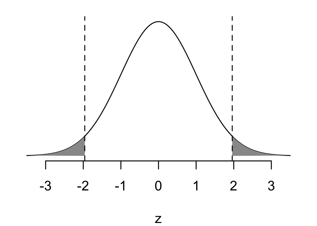
When the null hypothesis is true, z follows the standard normal distribution, with a mean of 0 and a standard deviation of 1. For a two-tailed test with \alpha = .05, the critical values of z are \pm 1.96: 2.5% of the area under the curve lies above 1.96 and 2.5% below -1.96 (Figure 10.2). A value of z in one of these two rejection regions is unlikely if H0 is true, and H0 is rejected. For a one-tailed test, the whole 5% is placed in one tail, and the critical value is 1.645 or -1.645, depending on the direction stated in H1.
Of note is the fact that the direction of a one-tailed test must be stated before the data is collected, based on theory or on previous research. Choosing the direction after seeing which way the sample mean falls doubles the real chance of a Type I error.
10.1.3 An Example
A math placement test is taken by all students admitted to a university. In the population of admitted students, the test has a mean of 70 points and a standard deviation of 12. A group of 36 students attended a summer bridge program before starting university. The question asked is: Did the students in the bridge program score differently on the placement test than the population of admitted students? The data set66 Column labels are: student and score. was made up for this example.
6 Column labels are: student and score.
   Min. 1st Qu.  Median    Mean 3rd Qu.    Max.
  51.00   66.75   74.50   75.00   84.25   95.00
Hypotheses.
- Null hypothesis (H0): The mean placement score of the students in the bridge program is the same as the mean of the population (\mu = 70).
- Alternative hypothesis (H1): The mean placement score of the students in the bridge program is different from the mean of the population (\mu \neq 70).
The test is two-tailed77 The program is meant to help the students, but it may also attract students who are less prepared than the others. There is no strong reason to expect a direction..
7 The program is meant to help the students, but it may also attract students who are less prepared than the others. There is no strong reason to expect a direction.
Decision criteria. The significance level is set at \alpha = .05. H0 is rejected if z is larger than 1.96 or smaller than -1.96, or, equivalently, if the p-value is smaller than \alpha. The effect size is Cohen’s d, the difference between the two means divided by the standard deviation of the population.
The z test has the same assumptions as the one-sample t-Test, with one addition: the standard deviation of the population must be known. With 36 students, the central limit theorem ensures that the sampling distribution of the mean is approximately normal.
The mean score of the students in the bridge program is 75.00. The standard error is 12 / \sqrt{36} = 2.00, and therefore:
z = \frac{\bar{x} - \mu}{\sigma / \sqrt{n}} = \frac{75.00 - 70}{2.00} = 2.50
[1] 2.5[1] 0.01241933Decision. With z = 2.50, p = .012, the computed value is larger than the critical value of 1.96, and the p-value is smaller than \alpha = .05. The null hypothesis is rejected and the alternative hypothesis accepted: the students in the bridge program scored differently from the population of admitted students. The positive value of z shows that they scored higher.
The 95% confidence interval for the mean of the bridge students, \bar{x} \pm 1.96 \times \sigma_{\bar{x}}, runs from 71.08 to 78.92, and does not include the population mean of 70.
Effect size. Cohen’s d = (75.00 - 70) / 12 = 0.42, a small to medium effect. The students in the bridge program scored, on average, 5.00 points higher than the population.
Of note is the fact that the students chose to attend the program. The result shows that they scored higher, not that the program made them score higher88 Students who choose to attend a bridge program may also be more motivated than others. See A Few Words About Causality..
8 Students who choose to attend a bridge program may also be more motivated than others. See A Few Words About Causality.
Here is an example of how to write up the results:
A one-sample z test compared the math placement scores of 36 students who attended a summer bridge program with the population of admitted students (μ = 70, σ = 12). The students in the program scored significantly higher than the population (M = 75.00, 95% CI [71.08, 78.92]), z = 2.50, p = .012, d = 0.42.
10.1.4 From z to t
The z test needs \sigma, the standard deviation of the population. When it is not known, which is the usual situation, it has to be estimated from the sample, using s. The estimate adds uncertainty, especially in small samples, and the resulting statistic no longer follows the normal distribution. It follows the t distribution, which has heavier tails than the normal distribution and depends on the degrees of freedom. As the sample grows, s becomes a better estimate of \sigma, and the t distribution comes closer to the normal distribution99 With 30 degrees of freedom, for example, the two-tailed critical value of t is 2.04, compared with 1.96 for z.. This is the statistic used by the t-Tests in the rest of the chapter.
9 With 30 degrees of freedom, for example, the two-tailed critical value of t is 2.04, compared with 1.96 for z.
10.2 One-Sample t-Test
At a glance
- Question
- Does the mean of a group differ from a reference value?
- Design
- One group, one measurement, compared with a value that does not come from the data
- Dependent variable
- Interval or ratio
- Assumptions
-
- Independent observations: each participant is measured once
- Randomly selected sample
- DV normally distributed (less critical in larger samples)
- Null hypothesis
- The population mean equals the reference value (\mu = \mu_{0})
- Test statistic
- t, with n - 1 degrees of freedom
- Effect size
- Cohen’s d: 0.2 small, 0.5 medium, 0.8 large
- If conditions fail
-
- The DV is ordinal, or clearly not normal in a small sample → One-sample Wilcoxon signed-rank test
- The distribution is also clearly skewed, or only above or below the value is known → Sign test
- Include in the write-up
-
- The sample size, mean, and standard deviation, and the reference value
- The normality check: the scores did not depart significantly from normality (Shapiro-Wilk p = …)
- t(df) = …, p = …, with the 95% CI of the mean
- Cohen’s d
Used when the mean of a sample is compared with a reference value that does not come from the data itself1010 E.g., a population mean reported in official statistics, the norm published for a standardized test, an industry standard, or a value predicted by theory.. For example, the one-sample t-Test is used when we want to know if the students of a school score, on average, differently from the national average on a standardized test.
10 E.g., a population mean reported in official statistics, the norm published for a standardized test, an industry standard, or a value predicted by theory.
The following assumptions must be met to use the one-sample t-Test:
- DV measured on an interval or ratio scale;
- Independent observations, a participant’s score should not be affected by another participant’s score;
- Randomly selected sample;
- Normally distributed data1111 With larger samples the test is fairly robust to moderate departures from normality..
11 With larger samples the test is fairly robust to moderate departures from normality.
If the standard deviation of the population is known, the z test can be used instead. However, in most real-life situations the population standard deviation is not known, and the t-Test estimates it from the sample.
An example: a university recommends that students spend 12 hours per week on independent study for each three-credit course. An instructor asks the 40 students enrolled in such a course how many hours they studied in a typical week. The question asked is: Do the students study as much as the university recommends? The data set was made up for this example. An excerpt of the data is presented in Table 10.2.
| Student | Hours |
|---|---|
| 1 | 9.7 |
| 2 | 6.8 |
| 3 | 13.1 |
| 4 | 10.7 |
| 5 | 4.6 |
| 6 | 5.3 |
Hypotheses. The reference value is the recommended 12 hours (\mu_{0} = 12).
- Null hypothesis (H0): In the population of students, the mean study time is 12 hours per week (\mu = 12).
- Alternative hypothesis (H1): In the population of students, the mean study time is different from 12 hours per week (\mu \neq 12).
Because the students could study either more or less than recommended, H1 does not state a direction and the test is two-tailed.
Decision criteria. The significance level is set at \alpha = .05. The degrees of freedom are the sample size minus one, in this case 40 - 1 = 39. H0 is rejected if the p-value is smaller than \alpha. The effect size is Cohen’s d, the difference between the sample mean and the reference value divided by the standard deviation of the sample.
As always, it is helpful to familiarize ourselves with the data first. Let’s take a look at some summary statistics.
   Min. 1st Qu.  Median    Mean 3rd Qu.    Max.
  3.300   9.025  10.600  10.703  13.100  19.000
[1] 3.3669210.2.1 Testing Assumption of Normality
    Shapiro-Wilk normality test

data:  sh$hours
W = 0.9797, p-value = 0.6785
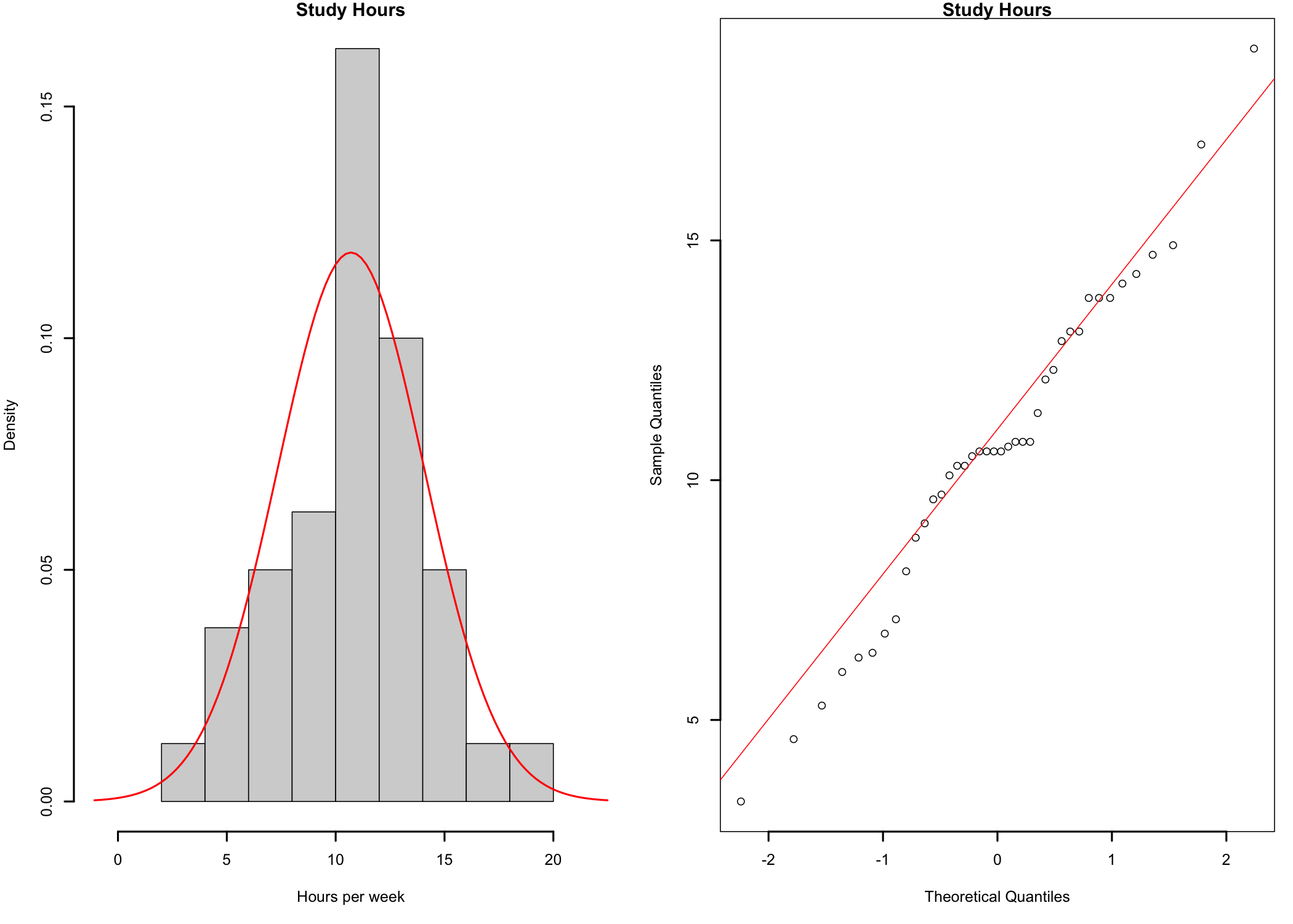
Both the histogram and the qq-plot (Figure 10.3) suggest that the data is relatively close to a normal distribution, with no significant departures. The Shapiro-Wilk test supports the same conclusion (p = .678 > .05), and therefore there is no reason to doubt the assumption of normality.
10.2.2 The t-Test
Before running the test, let’s see how the t statistic is computed. It is the difference between the sample mean and the reference value, divided by the standard error of the mean1212 The standard deviation of the sample divided by the square root of the sample size.:
12 The standard deviation of the sample divided by the square root of the sample size.
t = \frac{\bar{x} - \mu_{0}}{s / \sqrt{n}} = \frac{10.70 - 12}{3.37 / \sqrt{40}} = -2.44
A negative value of t indicates that the sample mean is lower than the reference value.
    One Sample t-test

data:  sh$hours
t = -2.4373, df = 39, p-value = 0.01946
alternative hypothesis: true mean is not equal to 12
95 percent confidence interval:
  9.625707 11.779293
sample estimates:
mean of x
  10.7025
Decision. With t(39) = -2.44, p = .019, the p-value is smaller than \alpha = .05. The null hypothesis is rejected and the alternative hypothesis accepted: the mean study time of the students is different from the recommended 12 hours. The negative value of t shows that they study less than recommended.
The same decision can be reached in two other ways, which help understand what the test does:
- Using the critical value. For a two-tailed test with \alpha = .05 and 39 degrees of freedom, the critical values of t are \pm 2.02. They define the interval inside which the values of t are likely to be observed if the null hypothesis is true. The computed value (t = -2.44) falls outside this interval, and therefore H0 is rejected.
- Using the confidence interval. The 95% confidence interval for the mean study time is between 9.63 and 11.78 hours. The reference value of 12 hours is outside the interval, which suggests that it is not a plausible value for the population mean.
Effect size. Cohen’s d = -0.39 indicates that the students study about 0.4 standard deviations less than recommended, an effect between small and medium. In real-life terms, the students study, on average, 1.30 hours per week less than recommended.
Finally, here is an example of how to write up the results in a publication.
A one-sample t-Test compared the weekly independent study time of 40 students with the 12 hours recommended by the university. The study times did not depart significantly from normality (Shapiro-Wilk p = .678). The students studied significantly less than recommended (M = 10.70, SD = 3.37, 95% CI [9.63, 11.78]), t(39) = -2.44, p = .019, d = -0.39.
10.3 The One-Sample Wilcoxon Signed-Rank Test
At a glance
- Use instead of
- The one-sample t-Test, when the DV is ordinal or clearly not normal in a small sample
- Question
- Does the median of a group differ from a reference value?
- Design
- One group, one measurement, compared with a reference value
- Dependent variable
- Ordinal, interval, or ratio
- Assumptions
-
- Independent observations: each participant is measured once
- The scores are distributed symmetrically around their median
- The distances from the reference value can be ranked by their size
- Null hypothesis
- The population median equals the reference value
- Test statistic
- V, the sum of the ranks of the scores above the reference value
- Effect size
- Matched-pairs rank-biserial correlation, rrb: .10 small, .30 medium, .50 large
- If conditions fail
-
- The distribution is clearly skewed → Sign test
- Include in the write-up
-
- The sample size and median, and the reference value
- Why the rank-based test was used
- V = …, p = …
- rrb
The rank-based alternative to the one-sample t-Test. It is used when the DV is ordinal1313 The test ranks the distances by their size, so the distances between the categories must be at least roughly comparable, as on a rating scale. When they are not, the sign test, which uses only the direction of each distance, is the safer choice., or when it is measured on an interval or ratio scale but is clearly not normally distributed. Instead of the mean, the test looks at the median. The distance between each score and the reference value is computed, and the distances are ranked by their size, ignoring their sign. The ranks of the positive distances and the ranks of the negative distances are then added up separately. If the median is equal to the reference value, the two sums should be about the same.
13 The test ranks the distances by their size, so the distances between the categories must be at least roughly comparable, as on a rating scale. When they are not, the sign test, which uses only the direction of each distance, is the safer choice.
The test assumes that the scores are distributed symmetrically around their median1414 When the distribution is clearly skewed, the sign test makes no such assumption.. Let’s run it on the study hours of the 40 students.
14 When the distribution is clearly skewed, the sign test makes no such assumption.
Hypotheses.
- Null hypothesis (H0): In the population of students, the median study time is 12 hours per week.
- Alternative hypothesis (H1): In the population of students, the median study time is different from 12 hours per week.
Decision criteria. The significance level is set at \alpha = .05, and the test is two-tailed. The test statistic, V, is the sum of the ranks of the positive distances. H0 is rejected if the p-value is smaller than \alpha. The effect size is the matched-pairs rank-biserial correlation, r_{rb}, the difference between the sums of the positive and of the negative ranks, divided by the sum of all ranks. It ranges from -1 (all scores below the reference value) to 1 (all scores above it), and is read with the same guidelines as a correlation: .10 small, .30 medium, .50 large.
    Wilcoxon signed rank test with continuity correction

data:  sh$hours
V = 244, p-value = 0.02608
alternative hypothesis: true location is not equal to 12
Decision. With V = 244, p = .026, the p-value is smaller than \alpha = .05 and H0 is rejected: the median study time of the students (Mdn = 10.6 hours) is different from the recommended 12 hours.
Effect size. r_{rb} = -0.40, a medium effect. The negative sign shows that most of the students study less than recommended.
The Wilcoxon test leads to the same conclusion as the t-Test. When the assumptions of the t-Test are met, as in this example, the t-Test is preferred, because it uses the scores themselves rather than their ranks and therefore has more power to detect a difference.
A one-sample Wilcoxon signed-rank test compared the weekly independent study time of 40 students with the 12 hours recommended by the university. The median study time (Mdn = 10.6) was significantly lower than recommended, V = 244, p = .026, rrb = -.40.
10.4 Independent Samples t-Test
At a glance
- Question
- Do the means of two independent groups differ?
- Design
- Two independent groups, one measurement of each participant
- Dependent variable
- Interval or ratio
- Independent variable
- Nominal, two levels
- Assumptions
-
- Independent observations: each participant belongs to one group only
- DV normally distributed in each group (less critical in larger samples)
- Null hypothesis
- The two population means are equal (\mu_{1} = \mu_{2})
- Test statistic
- t
- Effect size
- Cohen’s d: 0.2 small, 0.5 medium, 0.8 large
- If conditions fail
-
- The variances are not equal → Welch’s version of the t-Test, the default in this book
- The DV is ordinal, or clearly not normal in a small sample → Mann-Whitney U test
- The question is about the medians, and the two distributions have different shapes → Mood’s median test
- Include in the write-up
-
- The size of each group, and its mean and standard deviation
- The assumption checks, for example: the scores did not depart significantly from normality in either group (Shapiro-Wilk p = …)
- The version of the test (Welch’s, unless the variances are equal)
- t(df) = …, p = …
- Cohen’s d
Used when the observations collected under one treatment condition are not related to the observations collected under the other treatment condition. For example, the independent samples t-Test is used when randomly selected subjects are exposed to two different experimental conditions (IV) and we want to know if the two groups are or are not different on some characteristic (DV).
The following assumptions must be met to use the independent samples t-Test:
- Normally distributed data.
- Randomly selected samples;
- Samples are independent;
Data normality can be verified by looking at the distribution of the data (histograms) or through a test of normality. F or Levene’s tests can be used to test equality of variances.
The test computes how likely it would be to observe a difference between the two sample means at least as large as the one found if, in the population, there were no difference between the means (the null hypothesis). This probability is the p-value reported by the t-Test. A small p-value means that the observed difference would be unusual if the null hypothesis were true.
An example: consider studying the differences in height between males and females of the homo sapiens species. We measure 100 individuals, 50 females (F) and 50 males (M). An excerpt of the height measurement data is presented in Table 10.3.
| Gender | Height |
|---|---|
| F | 67 |
| F | 67 |
| F | 60 |
| M | 72 |
| M | 71 |
| M | 67 |
Hypotheses.
- Null hypothesis (H0): In the population there is no difference between male and female heights (\mu_{M} = \mu_{F}).
- Alternative hypothesis (H1): In the population, male and female heights differ (\mu_{M} \neq \mu_{F}).
Decision criteria. The significance level is set at \alpha = .05. The test is two-tailed, because H1 does not state which group is taller. R runs Welch’s version of the t-Test by default, which does not require the two groups to have equal variances. H0 is rejected if the p-value is smaller than \alpha.
The first step in data analysis is to familiarize oneself with the data. So, let’s take a look at the some summary statistics.
    Gender              Height
 Length:100         Min.   :60.00
 Class :character   1st Qu.:67.00
 Mode  :character   Median :69.00
                    Mean   :69.41
                    3rd Qu.:72.25
                    Max.   :79.00
10.4.1 Testing Assumption of Normality
As an example, we will work through the most common options to test the normality of a dataset.
Distributions
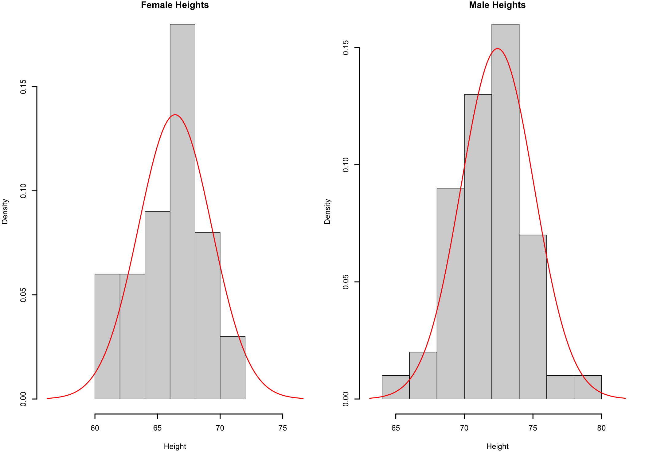
Based on the histogram plots (Figure 10.4) the data seems to be relatively close to a bell-shaped distribution1515 The histograms for Males and Females may look different because of possible differences between the number of bars used to represent the data. This is due to the way R computes the number of bins to use for data representation of a data set.. In this case, while the resemblance to a bell shape may be more difficult to observe, it is because of the small number of data points available for analysis. The more data points in the sample, if the sample distribution is close to the normal distribution, the closer the histogram would be to the bell-shaped curve of the normal distribution. While the visual checks are fine, let’s take a closer look at sample data normality.
15 The histograms for Males and Females may look different because of possible differences between the number of bars used to represent the data. This is due to the way R computes the number of bins to use for data representation of a data set.
qq-Plots
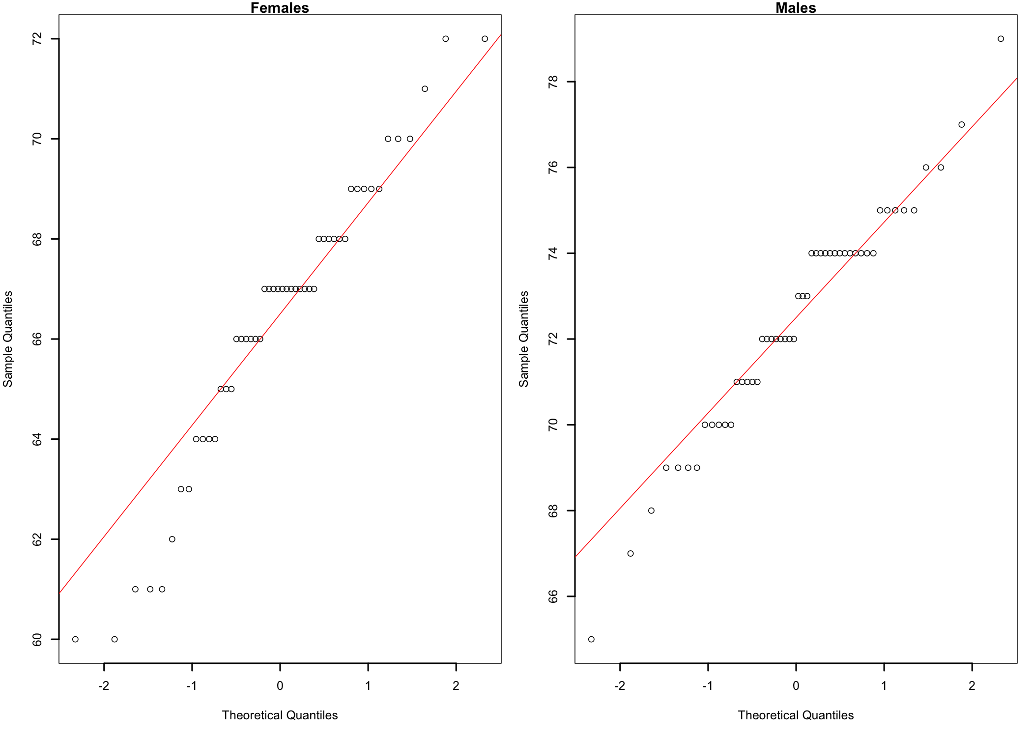
As Figure 10.5 shows, the data points form a fairly straight line for both males and females, which suggests that the heights in both groups are close to a normal distribution. The slight S-shaped curve is an indication of some departures from normality, but a visual inspection comparing the data points curves with the red straight diagonal lines suggests that these departures are small. Nevertheless, to be sure, let’s not rely on visual clues alone.
Skewness and Kurtosis
| Skewness | Kurtosis | |
|---|---|---|
| Females | -0.4309149 | 2.827522 |
| Males | -0.3149884 | 3.283505 |
The data in Table 10.4 shows that for females the data is slightly skewed to the left and playtkurtic (kurtosis < 3). The sample of males shows a similar situation. While numbers offer a bit more detail than visual representation, let’s go a step further and test data normality using a more specific statistical test.
Shapiro-Wilk Test
    Shapiro-Wilk normality test

data:  my.F
W = 0.95591, p-value = 0.05993
    Shapiro-Wilk normality test

data:  my.M
W = 0.96944, p-value = 0.2197
A p-value > 0.05 indicates that the null hypothesis cannot be rejected: neither sample departs significantly from a normal distribution. Together with the qq-plots, there is no reason to doubt the assumption of normality.
10.4.2 The t-Test
    Welch Two Sample t-test

data:  Height by Gender
t = -10.765, df = 97.193, p-value < 2.2e-16
alternative hypothesis: true difference in means between group F and group M is not equal to 0
95 percent confidence interval:
 -7.129868 -4.910132
sample estimates:
mean in group F mean in group M
          66.40           72.42
Decision. The output shows the probability p (p-value) that the t statistics would be this large or larger in absolute value (without the - sign) if the null hypothesis is true. For this analysis the value of p is so small1616 The value of the p-value is so small that R considers it, for the purpose of this test, indistinguishable from 0 and thus represented as 2.2e-16 (0.00000000000000022). R can represent smaller numbers, but for all intents and purposes, unless one needs to work with very, very small p-values, this value can be effectively considered equal to 0. that a difference this large would almost never occur if H0 were true. Because p is smaller than \alpha = .05, H0 is rejected: on average, there is a significant difference in height between males and females.
16 The value of the p-value is so small that R considers it, for the purpose of this test, indistinguishable from 0 and thus represented as 2.2e-16 (0.00000000000000022). R can represent smaller numbers, but for all intents and purposes, unless one needs to work with very, very small p-values, this value can be effectively considered equal to 0.
Effect size. A significant result says that a difference exists, not how large it is. For a t-Test, the effect size is Cohen’s d, the difference between the two means divided by their pooled standard deviation. Values around 0.2 indicate a small effect, 0.5 a medium effect, and 0.8 or more a large effect. Here d = 2.15: males and females differ in height by more than two standard deviations, a very large effect.
Finally, here is an example of how to write up the results in a publication.
An independent-samples t-Test compared the heights of 50 females and 50 males. Before the test, the assumptions were checked. The two groups are independent, because each participant belongs to only one of them. The heights did not depart significantly from normality in either group (Shapiro-Wilk, females: p = .060; males: p = .220). Equal variances were not assumed, so Welch’s version of the test was used. Males were significantly taller (M = 72.42, SD = 2.67) than females (M = 66.40, SD = 2.92), t(97.19) = 10.77, p < .001, d = 2.15.
10.5 The Mann-Whitney U Test
At a glance
- Use instead of
- The independent samples t-Test, when the DV is ordinal or clearly not normal in a small sample
- Question
- Do the scores of one of two independent groups tend to be higher?
- Design
- Two independent groups, one measurement of each participant
- Dependent variable
- Ordinal, interval, or ratio
- Independent variable
- Nominal, two levels
- Assumptions
-
- Independent observations: each participant belongs to one group only
- The test compares the medians only when the two distributions have the same shape
- Null hypothesis
- The scores of both groups come from the same distribution
- Test statistic
- U
- Effect size
- Rank-biserial correlation, rrb: .10 small, .30 medium, .50 large
- Include in the write-up
-
- The size of each group, and its median
- Why the rank-based test was used, for example an ordinal DV
- U = …, p = …
- rrb
The rank-based alternative to the independent samples t-Test1717 Also known as the Wilcoxon rank-sum test. The two names describe the same test.. It is used when the DV is ordinal, or when it is clearly not normally distributed in one or both groups. All the scores are ranked together, from the smallest to the largest, regardless of the group they belong to. If the groups do not differ, the high and the low ranks should be mixed evenly between them.
17 Also known as the Wilcoxon rank-sum test. The two names describe the same test.
The test statistic, U, has a simple meaning. Imagine pairing every female with every male, 50 \times 50 = 2500 pairs in all. U counts the pairs in which the female is taller1818 A tie, in which the two are equally tall, counts as half.. If heights did not differ between the genders, the female would be taller in about half of the pairs.
18 A tie, in which the two are equally tall, counts as half.
The test assumes that the two groups are independent. Of note is the fact that it compares the medians only when the two distributions have the same shape. Otherwise, it tests something broader: whether the scores of one group tend to be higher than the scores of the other.
Hypotheses.
- Null hypothesis (H0): In the population, male and female heights have the same distribution. A randomly chosen female is as likely to be taller than a randomly chosen male as to be shorter.
- Alternative hypothesis (H1): In the population, the heights of one gender tend to be higher than the heights of the other.
Decision criteria. The significance level is set at \alpha = .05, and the test is two-tailed. H0 is rejected if the p-value is smaller than \alpha. The effect size is the rank-biserial correlation, r_{rb} = 1 - 2U / (n_{1}n_{2}), read with the same guidelines as a correlation: .10 small, .30 medium, .50 large.
    Wilcoxon rank sum test with continuity correction

data:  Height by Gender
W = 150.5, p-value = 2.839e-14
alternative hypothesis: true location shift is not equal to 0
Decision. With U = 150.5, p < .001, H0 is rejected: the heights of males (Mdn = 72.5) tend to be higher than the heights of females (Mdn = 67.0).
Effect size. The female is taller in only 6% of the 2500 female-male pairs. The rank-biserial correlation, r_{rb} = 0.88, indicates a large effect.
As with the one-sample test, the t-Test is preferred when its assumptions are met.
A Mann-Whitney U test compared the heights of 50 females and 50 males. Males (Mdn = 72.5) were significantly taller than females (Mdn = 67.0), U = 150.5, p < .001, rrb = .88.
10.6 Mood’s Median Test
At a glance
- Use instead of
- The Mann-Whitney U test, when the question is about the medians and the two distributions have different shapes
- Question
- Do the medians of two independent groups differ?
- Design
- Two independent groups, one measurement of each participant
- Dependent variable
- Ordinal, interval, or ratio
- Independent variable
- Nominal, two levels
- Assumptions
-
- Independent observations: each participant belongs to one group only
- Expected counts of 5 or more in each cell of the table of counts above and below the grand median
- Null hypothesis
- The two population medians are equal
- Test statistic
- \chi^{2}, with one degree of freedom
- Effect size
- Phi (\phi): .10 small, .30 medium, .50 large
- If conditions fail
-
- Expected counts below 5 → Fisher’s exact test on the same table
- Include in the write-up
-
- The size of each group, and its median
- The grand median, and how scores equal to it were counted
- \chi^{2}(1, N = …) = …, p = …
- Phi
When the question is about the medians, and the two distributions do not have the same shape, Mood’s median test compares the medians directly. The median of all the scores together, the grand median, is computed first. Each score is then classified as above the grand median or not, and the counts are compared between the two groups with a chi-square test of independence. If the two groups have the same median, about half of the scores of each group should fall above the grand median.
Hypotheses.
- Null hypothesis (H0): In the population, the median heights of males and females are the same.
- Alternative hypothesis (H1): In the population, the median heights of males and females differ.
Decision criteria. The significance level is set at \alpha = .05. H0 is rejected if the p-value of the chi-square test is smaller than \alpha. Like any chi-square test, it requires independent observations and expected counts of 5 or more in each cell of the table1919 See When the Expected Counts Are Too Small.. With small groups, Fisher’s exact test can be run on the same table instead. The effect size is phi (\phi), read with the same guidelines as a correlation.
      Height
Gender Above At or below
     F     6          44
     M    43           7
    Pearson's Chi-squared test with Yates' continuity correction

data:  my.mt
X-squared = 51.861, df = 1, p-value = 5.958e-13
The grand median is 69. The smallest expected count is 24.5, well above 5. The 9 heights equal to the median were counted as at or below it2020 Some authors leave such scores out. When many scores are tied at the median, the choice can change the result..
20 Some authors leave such scores out. When many scores are tied at the median, the choice can change the result.
Decision. With \chi^{2}(1) = 51.86, p < .001, H0 is rejected: the median heights of males and females differ. 86% of the males are above the grand median, compared with 12% of the females.
Effect size. \phi = 0.74, a large effect.
Mood’s median test makes the fewest assumptions of the three tests, but it also has the least power. It keeps only whether each score is above or below the grand median and discards everything else. The t-Test uses the scores, the Mann-Whitney test their ranks, and Mood’s test only their side of the median.
10.7 Paired Samples t-Test
At a glance
- Question
- Do two related measurements differ on average?
- Design
- One group measured twice, or matched pairs
- Dependent variable
- Interval or ratio
- Independent variable
- The two measurements or conditions
- Assumptions
-
- The observations are paired in a meaningful way
- Each pair is independent of the others
- The differences are normally distributed (the scores themselves need not be)
- Null hypothesis
- The mean of the differences is zero (\mu_{D} = 0)
- Test statistic
- t, with the number of pairs - 1 degrees of freedom
- Effect size
- Cohen’s dz, the mean of the differences divided by their standard deviation: 0.2 small, 0.5 medium, 0.8 large
- If conditions fail
-
- The DV is ordinal, or the differences are clearly not normal in a small sample → Wilcoxon signed-rank test
- The differences are also clearly skewed, or only the direction of each change is known → Sign test
- The DV has two categories, such as Yes and No → McNemar’s test
- Include in the write-up
-
- The number of pairs, and the mean and standard deviation of each measurement
- The normality check of the differences (Shapiro-Wilk p = …)
- t(df) = …, p = …
- Cohen’s dz, and the mean difference with its 95% CI
The paired-samples t-Test is used when the observation collected from one group is related in some way to the corresponding observation in the second group. Some examples of studies where this test would be appropriate:
- A study using repeated measures in which case some characteristic is measured for the same participants before and after a treatment. In this case, because the participants are the same, an observation before the treatment will have a corresponding observation after the treatment, with the correspondence being provided by the participant.
- A variant of the above is a pretest-posttest study, where there is a test given to the participants before the intervention, and then another test is given after the intervention.
- A study in which the participants are assigned to the treatment groups using some type of matching procedure or process. That is, one participant is exposed to one of the experimental conditions while another participant, selected using a matching procedure is exposed to the other experimental treatment.
- A study in which each participant is exposed to both treatment conditions.
Assumptions underlying paired-samples t-test:
- DV - interval or ratio;
- Observations should be paired in some meaningful way2121 E.g., two measurements of the same participant, or one measurement for each participant in a matched pair.;
21 E.g., two measurements of the same participant, or one measurement for each participant in a matched pair.
- Independent observations, a participant’s score in one treatment should not be affected by another participant’s score(s);
- Random sampling drawn from population;
- Normal distribution of difference scores2222 The two sets of scores do not need to be normally distributed on their own, and their variances do not need to be equal, because the test uses only the differences..
22 The two sets of scores do not need to be normally distributed on their own, and their variances do not need to be equal, because the test uses only the differences.
The test reduces each pair of observations to a single value, the difference between the two scores, and then looks at whether the mean of these differences is far enough from zero. In this way the participants act as their own controls. Whatever stays the same for a participant from one measurement to the other2323 For example, the participant’s general ability. cancels out in the difference.
23 For example, the participant’s general ability.
An example: a school runs a six-week tutoring program in reading. Before the program, 30 students take a reading comprehension test, scored from 0 to 50. After the program, the students take a parallel form of the same test. The question asked is: Did the reading scores of the students change after the program? The data set was made up for this example. An excerpt of the data is presented in Table 10.5.
| Student | Before | After |
|---|---|---|
| 1 | 42 | 44 |
| 2 | 38 | 36 |
| 3 | 26 | 37 |
| 4 | 22 | 17 |
| 5 | 24 | 25 |
| 6 | 33 | 40 |
Hypotheses. The paired-samples t-Test works with the difference between the two observations in each pair. In this case, the difference is the score after the program minus the score before the program (D = after - before). A positive difference means that the student improved.
- Null hypothesis (H0): In the population, the mean of the differences is zero (\mu_{D} = 0). That is, on average, the scores before and after the program are the same.
- Alternative hypothesis (H1): In the population, the mean of the differences is not zero (\mu_{D} \neq 0). That is, on average, the scores changed.
If theory predicts the direction of the change, H1 can be one-tailed2424 For example, \mu_{D} > 0 when the scores are expected to increase.. However, a program can also make things worse, so this example keeps a two-tailed H1.
24 For example, \mu_{D} > 0 when the scores are expected to increase.
Decision criteria. The significance level is set at \alpha = .05, and the test is two-tailed. The degrees of freedom are the number of pairs minus one, in this case 30 - 1 = 29. H0 is rejected if the p-value is smaller than \alpha. The effect size is Cohen’s dz, the mean of the differences divided by their standard deviation, read with the same guidelines as Cohen’s d.
As always, let’s first take a look at some summary statistics, including those of the differences.
     before       after            diff
 Min.   :13   Min.   :16.00   Min.   :-7.000
 1st Qu.:25   1st Qu.:27.25   1st Qu.: 0.250
 Median :31   Median :34.50   Median : 4.000
 Mean   :30   Mean   :33.07   Mean   : 3.067
 3rd Qu.:33   3rd Qu.:40.00   3rd Qu.: 6.000
 Max.   :44   Max.   :49.00   Max.   :13.000
10.7.1 Testing Assumption of Normality
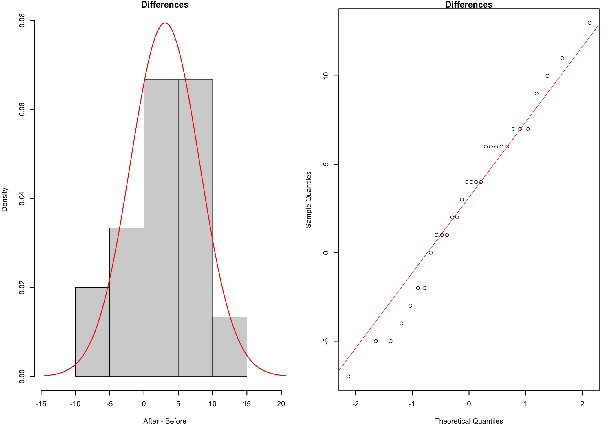
Of note is the fact that the assumption refers to the differences, not to the two sets of scores. Therefore, the normality checks are run on the differences.
    Shapiro-Wilk normality test

data:  tut$diff
W = 0.97594, p-value = 0.7104
Both the histogram and the qq-plot (Figure 10.6) suggest that the differences are relatively close to a normal distribution, with no significant departures. The Shapiro-Wilk test supports the same conclusion (p = .710 > .05), and therefore there is no reason to doubt the assumption of normality.
10.7.2 The t-Test
The t statistic is the mean of the differences divided by its standard error2525 The standard deviation of the differences divided by the square root of the number of pairs.. In other words, the paired-samples t-Test is a one-sample t-Test run on the differences, with a reference value of zero:
25 The standard deviation of the differences divided by the square root of the number of pairs.
t = \frac{\bar{D}}{s_{D} / \sqrt{n}} = \frac{3.07}{5.02 / \sqrt{30}} = 3.34
The output of the paired-samples t-Test shows the same value of t, together with its p-value and the confidence interval for the mean difference.
    Paired t-test

data:  tut$after and tut$before
t = 3.3436, df = 29, p-value = 0.002293
alternative hypothesis: true mean difference is not equal to 0
95 percent confidence interval:
 1.190815 4.942518
sample estimates:
mean difference
       3.066667
Decision. With t(29) = 3.34, p = .002, the p-value is smaller than \alpha = .05. The null hypothesis is rejected and the alternative hypothesis accepted: on average, the reading scores changed between the two tests. The mean difference is positive (3.07 points, 95% CI 1.19 to 4.94), which means that the scores increased.
Effect size. Cohen’s dz = 0.61 indicates that the average gain is about 0.6 standard deviations of the differences, a medium effect.
Of note is the fact that a significant change in a single group does not show that the program caused the change. The students may have improved anyway over the six weeks, or may have done better the second time because they were familiar with the test. A comparison group, not exposed to the program, would be needed to rule out these explanations (see the problems listed below).
Finally, here is an example of how to write up the results in a publication.
A paired-samples t-Test compared the reading comprehension scores of 30 students before and after a six-week tutoring program. The differences between the two scores did not depart significantly from normality (Shapiro-Wilk p = .710). Scores were significantly higher after the program (M = 33.07, SD = 9.25) than before it (M = 30.00, SD = 6.94), t(29) = 3.34, p = .002, dz = 0.61. The mean gain was 3.07 points (95% CI [1.19, 4.94]).
Paired-samples t-tests problems:
- The designs that utilize this type of t-test are many times fairly weak2626 For example, a before-and-after study without a comparison group cannot separate the effect of the treatment from other changes that happen over the same time..
26 For example, a before-and-after study without a comparison group cannot separate the effect of the treatment from other changes that happen over the same time.
- The experiment can have many confounding variables, such as the order of treatments for a study in which each participant is exposed to both treatment conditions, in which case it could be difficult to determine if the outcomes are because of the treatment conditions themselves, due to the order of treatments, or a combination of both.
- Repeated measures tests can also show significant confounding, especially for those that span a significant amount of time (e.g., a semester) over which things that happen outside the treatment conditions can influence the outcome.
10.8 The Wilcoxon Signed-Rank Test
At a glance
- Use instead of
- The paired samples t-Test, when the DV is ordinal or the differences are clearly not normal in a small sample
- Question
- Do two related measurements differ?
- Design
- One group measured twice, or matched pairs
- Dependent variable
- Ordinal, interval, or ratio
- Assumptions
-
- The observations are paired, and each pair is independent of the others
- The differences are distributed symmetrically around their median, and can be ranked by their size
- Null hypothesis
- The median of the differences is zero
- Test statistic
- V, the sum of the ranks of the positive differences (differences of zero are left out)
- Effect size
- Matched-pairs rank-biserial correlation, rrb: .10 small, .30 medium, .50 large
- If conditions fail
-
- The differences are clearly skewed → Sign test
- Include in the write-up
-
- The number of pairs, and the median of each measurement
- Why the rank-based test was used
- V = …, p = …
- rrb
The rank-based alternative to the paired samples t-Test. It works like the one-sample Wilcoxon test, run on the differences with a reference value of zero. The differences are ranked by their size, ignoring their sign, and the ranks of the positive and of the negative differences are added up separately. Differences of zero carry no information about the direction of the change and are left out. The test assumes that the differences are distributed symmetrically around their median, and that they can be ranked by their size, which an ordinal scale does not always allow2727 When only the direction of each change is meaningful, the sign test is the safer choice..
27 When only the direction of each change is meaningful, the sign test is the safer choice.
Hypotheses.
- Null hypothesis (H0): In the population, the median of the differences is zero. The scores are as likely to go up as to go down.
- Alternative hypothesis (H1): In the population, the median of the differences is not zero.
Decision criteria. The significance level is set at \alpha = .05, and the test is two-tailed. H0 is rejected if the p-value is smaller than \alpha. The effect size is the matched-pairs rank-biserial correlation, r_{rb}.
    Wilcoxon signed rank test with continuity correction

data:  tut$after and tut$before
V = 349, p-value = 0.004538
alternative hypothesis: true location shift is not equal to 0
1 student had the same score on both tests, which leaves 29 differences.
Decision. With V = 349, p = .005, H0 is rejected: the reading scores changed after the program. The median gain was 4.0 points.
Effect size. r_{rb} = 0.60, a large effect. The positive sign shows that the scores went up for most students.
A Wilcoxon signed-rank test compared the reading comprehension scores of 30 students before and after a six-week tutoring program. Scores were significantly higher after the program (Mdn = 34.5) than before it (Mdn = 31.0), V = 349, p = .005, rrb = .60.
10.9 The Sign Test
At a glance
- Use instead of
- The paired samples t-Test or the Wilcoxon signed-rank test, when the differences are clearly skewed or only their direction is known; also for one group against a reference value
- Question
- Do the scores go up more often than they go down?
- Design
- One group measured twice, matched pairs, or one group compared with a reference value
- Dependent variable
- Any scale on which a change can be judged as up or down
- Assumptions
-
- The observations are paired, and each pair is independent of the others
- Null hypothesis
- Increases and decreases are equally likely (the proportion of increases is .5)
- Test statistic
- The number of increases, tested with a binomial test (changes of zero are left out)
- Effect size
- The proportion of increases, with its 95% CI
- Include in the write-up
-
- The number of pairs, and how many went up, down, or did not change
- The proportion of increases with its 95% CI, and p
The simplest test for paired data. It keeps only the direction of each difference: did the score go up or down? If H0 is true, a score is as likely to go up as to go down, and the number of increases follows a binomial distribution with a probability of .5. The sign test is therefore a binomial test on the number of increases2828 Like the Wilcoxon test, it leaves out the differences of zero..
28 Like the Wilcoxon test, it leaves out the differences of zero.
The sign test makes no assumption about the shape of the distribution of the differences. It can also be used when only the direction of the change is known, for example when an observer judges whether each participant got better or worse. The same test compares one group with a known value: the scores above and below the value are counted, in place of the increases and decreases.
Hypotheses.
- Null hypothesis (H0): In the population, the proportion of students whose score goes up is .5.
- Alternative hypothesis (H1): In the population, the proportion of students whose score goes up is not .5.
Decision criteria. The significance level is set at \alpha = .05, and the test is two-tailed. H0 is rejected if the p-value is smaller than \alpha. The effect size is the proportion of increases, with its confidence interval.
    Exact binomial test

data:  my.pos and my.n3
number of successes = 22, number of trials = 29, p-value = 0.00813
alternative hypothesis: true probability of success is not equal to 0.5
95 percent confidence interval:
 0.5645997 0.8970164
sample estimates:
probability of success
             0.7586207
Decision. The scores went up for 22 of the 29 students and down for 7, p = .008. H0 is rejected: more students improved than declined.
Effect size. The proportion of students who improved is 0.76 (95% CI [0.56, 0.90]).
The sign test has the least power of the paired tests, because it ignores how large each change is. A student who gained one point counts the same as a student who gained ten. The paired samples t-Test uses the size of the differences, the Wilcoxon test their ranks, and the sign test only their direction.
A sign test compared the reading comprehension scores of 30 students before and after a six-week tutoring program. Of the 29 students whose score changed, 22 improved, a proportion of .76 (95% CI [.56, .90]), p = .008.