5 Effect Size and Power

An experiment, or a study in general, should be designed to be sufficiently sensitive to be able to detect any differences the population may exhibit. The most direct ways to increase the sensitivity is to increase the sample size, by choosing treatments expected to produce large effects, and by reducing unexpected variance.

5.1 Relative Treatment Magnitude

The most popular measure of treatment magnitude is called omega squared (\omega^{2})11 Another measure used is the squared multiple-correlation coefficient, which represents how much of the total variation is associated with the variation in treatment.. It is a relative measure that reflects the portion (proportional amount) of population variance that can be attributed to the experimental treatment. That is, the proportion of variability explained by the treatment or, more commonly, explained variance. Its value is 0 if the treatment effects are absent in the population and has values between 0 and 1 if the effect is present.

Based on the value of \omega^{2}, in the behavioral sciences field, the effect size can be interpreted as (Cohen 1977):

• Small, for a value of .01;
• Medium, for a value of .06;
• Large, for a value of .15 or greater.

But how would one know whether the treatment is weak or not? Effects size, as measured by \omega^{2} is, basically, the ratio between the variance due to treatment and total variance (treatment + error). First, the actual effect size can only be estimated after the data is known. So, how would one estimate the treatment effect size at design stage? There are a few possibilities:

1. Deep knowledge of theory should be the primary source of information when estimating the potential strength of an intervention.

2. Search literature for independent variables that seem to produce large effects; use similar research published by others.

3. Choose the treatment and then run preliminary or pilot studies. Use the data to estimate the effect size for the main study. Eventually adjust treatment if needed.

In social sciences it is unlikely to observe large effect sizes22 Perception of effect size for the same treatment may differ between fields, researchers, and studies. This is why it is advisable to base any preliminary (at design time) estimates of effect size on theory and prior research as close to the desired field as possible, followed by pilot testing.. It is often the case that if a study has an IV that has large effects, that study is just the first step. Further refinements, looking as components of that first IV, will observe theoretical relevance for increasingly smaller effect sizes.

5.2 Standardized Effect Size33 The MyReLab website (https://www.myrelab.com) offers a more comprehensive power analysis tool.

Known as Cohen’s d, the standardized effect size represents the difference between the means of two groups divided by the Standard Deviation (SD), in absolute values.

d = \frac{|mean_{s1} - mean_{s2}|}{SD}

Fundamentally, Cohen’s d expresses the difference between two means in term of Standard Deviation units. It can be interpreted as an equivalent to a z-score for the standard normal distribution. Therefore, if the effect size is 0.6 (SDs above average) between group 1 and group 2, with mean of group 1 > mean of group 2, then the mean of group 1 exceeds about 73% of the values of group 244 Assuming both groups are normally distributed with the same standard deviation. The value is the share of the standard normal distribution below z = 0.6.. While unlikely to observe standardized effect sizes this large in real life, if its value is > 1, the difference between the two means is > 1 SD, while for d > 2, the difference between means is > 2 SDs.

According to Cohen and later Sawilowsky (Sawilowsky 2009), the standardized effect sizes can be thought of as:

• .01 - Very Small
• 0.2 - Small
• 0.5 - Medium
• 0.8 - Large
• 1.2 - Very Large
• 2.0 - Huge

Note: For independent groups, the Standard Deviation used to compute Cohen’s d is the pooled55 Pooled/combined/composite variance is based on the variance of multiple populations when the variance of the population is the same while the means may be different. Standard Deviation.

5.3 Controlling Type I and Type II Errors

In statistical analysis power is the probability the findings will reject a false null hypothesis. That is, when an effect is present, power is the likelihood that the effect is detected. So, why should the power of an experiment be controlled? First, because an experiment’s power represents the degree to which it can detect differences in treatment and the chances that the experiment can be replicated. Second, a power analysis will help avoid wasting resources when not necessary66 For example, adding more participants to a study can be costly in both time and money..

Overall, the statistical power of a test is determined by three factors:

• How large is the difference between the variables measured for the two or more groups involved in the study. A small difference produced by the treatment or cause will require a larger sample for the same power.
• What level of significance (\alpha) is set77 For example, 0.05, 0.01, or 0.001.. The lower \alpha, the lower the power for the same sample, and the larger the sample needed to keep it.

  7 For example, 0.05, 0.01, or 0.001.

• How many participants are in the study. The larger the sample, the higher the power for the same effect and significance level.

5.4 Controlling Power Through Sample Size

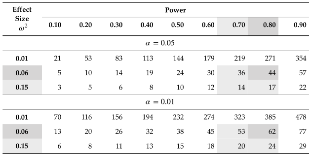
Power, Effect Size, and Significance influence the number of participants that are necessary to be able to observe differences between groups or variables of interest.

Figure 5.1 (adapted from Keppel (1991), p. 72) illustrates the relationship between Power, Effect Size, Significance, and Group Size. The number of participants needed (sample size) increases with the Power wanted, and decreases as the Effect Size and the Significance level increase. For example, for an Effect Size of .01 and an expected Power of .50 and \alpha of .05, the minimum number of participants in each group of the design would be 144. Therefore, if the study includes two groups, a control group and a treatment group, the entire sample size should be at least 288 participants. That is, the weaker the treatment, the more participants are needed to be able to observe the effects.

As a rule of thumb, when nothing better is known, a study should be designed for at least a medium Effect Size (\omega^2 = .06) and a relatively high Power (.70 or .80) for a Significance Level (\alpha) of .05. When theory or prior research points to a smaller effect that still matters, the study should be designed to detect that effect instead: a study planned for a medium effect has little power for a small one. A small effect size (weak treatment) requires considerably more resources to be able to observe the effect. Therefore, if possible, the intervention and/or variable(s) should be chosen to avoid weak treatments. Lower power is also to be avoided because it wastes resources (e.g., time, energy) to produce a significant result88 For example, for a power of .50 there is a 50-50 chance of observing significance.. Experiments with low power do not produce reliable findings. The sweet spot for the design of a study would be at the intersection of the highlighted columns and rows in the figure above.

5.4.1 Population vs. Sample

Population: Is the entire set or pool of similar individuals, items, or events of interest to a researcher. For example, all freshmen at a two-year college can represent a population. Another example would be all the wolves in the Yellowstone National Park. That is, the entire collection to be studied. Can be large or small, depending on the researcher’s interests.

Sample: A subset of individuals, items, or events, drawn from the population of interest. To continue the example above, 200 freshmen constitutes a sample. Or the 50 wolves researchers may have tagged with geo locators to follow their behavior. Because in many instances it may be impossible to cover the entire population, a sample allows researchers to use manageable numbers of subjects as representatives of the population to be studied. If the size and characteristics of the sample are appropriate, judgment calls or estimates can be made about the entire population.

5.5 Practical Advice on Sample Size

The purpose of computing the size of the minimum necessary sample at design time is to make sure the data is collected from enough participants to detect the effect of interest with the chosen power. A large sample does not make the results generalizable on its own. Whether they can be generalized back to the population depends on how the sample was drawn, and a sample that does not represent the population is not fixed by its size.

The table in figure 5.1 can be, for example, used for such a purpose. At the design phase, use prior studies, on the same subject or on similar or related topics, to estimate effect size (\omega^{2}) of the treatment intended to be administered. Then choose the level of significance (\alpha) you want (e.g., 0.05 or 0.01, or something else) and choose the power you wish your experiment to have. Based on the table you can then determine how many participants you should have, at the minimum, in each study group. So, if the experiment has, let’s say, two groups, if the table indicates that 30 participants are needed, at the minimum, per group, to observe the values you chose, you would need at least 60 participants in total, equally distributed between the two groups. But this is just a theoretical number.

This estimate is just the first step of the process. You should then consider the possibility that not all responses you receive (or measurements of the DV) will be usable, so it would be advisable to adjust upwards the value you calculate so that it is more likely to get the minimum number of usable responses.

Many of the tests work better if the groups are balanced (in number of participants). Therefore, the procedure for the selection of participants and assignment to the experimental groups should attempt to make that happen. And this is not just a matter of, say, assigning incoming participants (they come in randomly) alternatively to each study groups (treatment condition). You should also consider the type of treatment you are applying and the likelihood for the participant to drop early or to not complete the entire study.99 For example, the more complex and cognitively involved the task is, the more likely is for the participant to drop early, skip responses, or just guess, situations in which the experimenter ends up with missing or unusable data, or incomplete records.

In the end, the sample size determination is based both on numerical computation and the researcher’s understanding of the field and his or her grasp of how prior research fared. Usually, power estimates are based on the minimum effect size the researcher wishes to detect. A realistic estimate is usually based on prior research.

Below I listed resources that can help determine power and sample size. The first one is a software application that allow you to make the necessary computations. The second one is a resource that helps you understand how to use the R statistical computing language for the same purpose.

G*Power (http://www.gpower.hhu.de)

Power analysis in R (https://www.statmethods.net/stats/power.html).

MyReLab website (https://www.myrelab.com).