8 Assumptions and Outliers
Most statistical tests rely on a set of assumptions about the data they are used to analyze. These assumptions ensure that the test performs as expected and that the results can be interpreted with a high degree of confidence. Understanding when and how these assumptions lead to biases in analysis and what the consequences are is essential to meaningful data analysis.
For example, many tests assume that some part of the data is normally distributed: the DV within each group for the t-Test and the ANOVA, and the residuals for linear regression11 In a regression, the predictors and the criterion themselves do not need to be normally distributed. See Simple Linear Regression.. While these statistical tests vary in how well they can deal with departures from normality, if the data does not follow a normal distribution, the p-values and confidence intervals they compute may not be accurate, especially in small samples, and therefore it is important to check beforehand that the interpretation will be valid. In situations in which normality is not observed it is usually possible to find a different statistical test that is less sensitive to departures from normality.
1 In a regression, the predictors and the criterion themselves do not need to be normally distributed. See Simple Linear Regression.
What is important to remember is that each statistical test functions better when certain conditions, established by those who developed the test, are met. Therefore, assumptions need to be tested to make sure that the statistical test is appropriate to be used for the data set.
The most common parametric statistical analyses expect the data to be normally distributed and homogeneous.
8.1 Normality
Compares the sample’s distribution with the normal distribution (Figure 8.1).
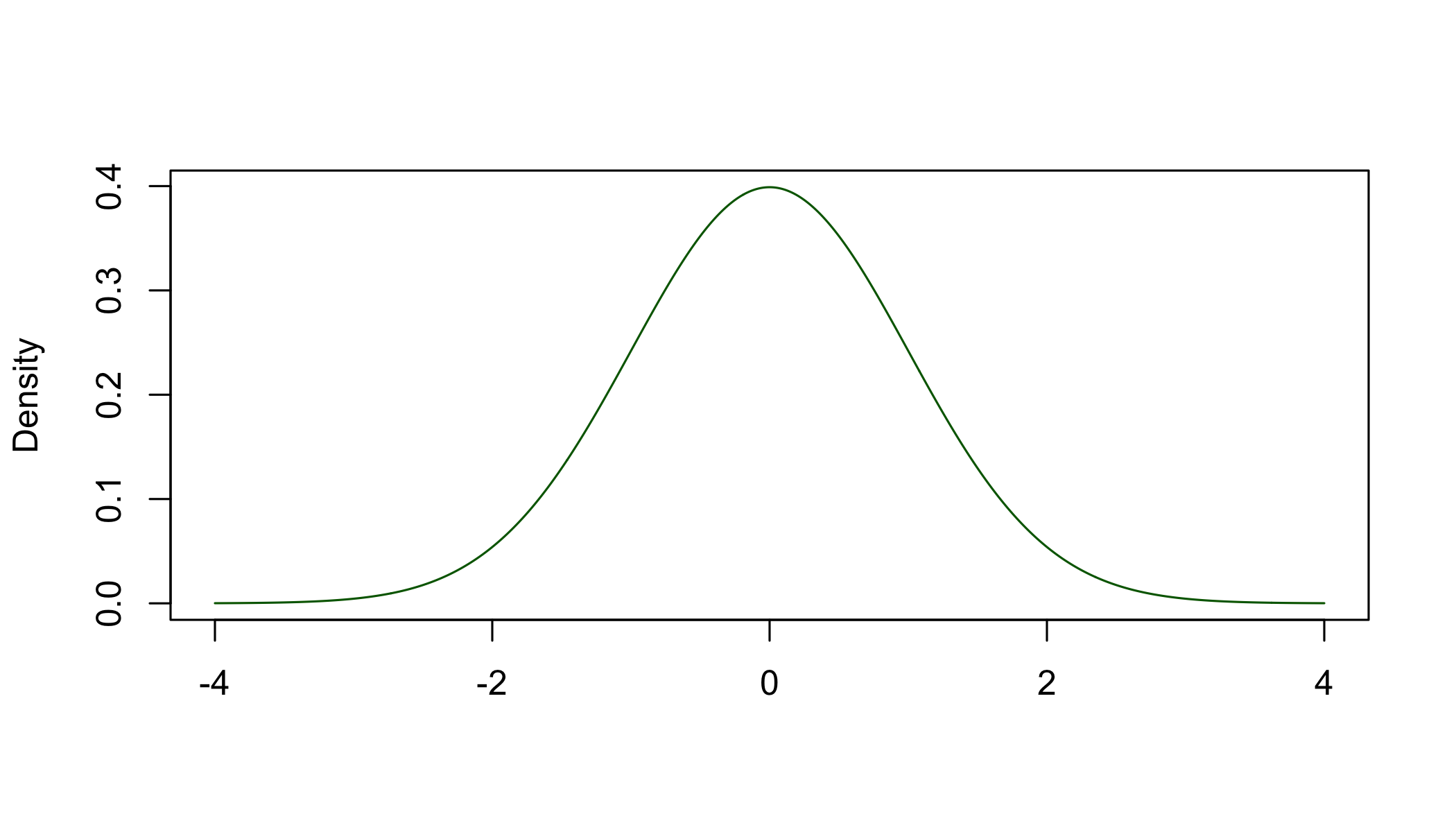
To study the normality of a data sample we use the skewness and kurtosis of the sample’s distribution to determine its departure from the theoretical normal distribution.
8.1.1 Moments of a Distribution
The shape of a distribution can be summarized by four numbers, called its moments. The first two are familiar22 See Describing Data.: the mean, which shows where the distribution is centered, and the variance, which shows how spread out it is. The third and the fourth describe its shape. They are computed from the deviations of the values from the mean, raised to the third and to the fourth power, and divided by the corresponding power of the standard deviation33 Dividing by a power of the standard deviation removes the units of the data, so that the shape of distributions measured on different scales can be compared.:
2 See Describing Data.
3 Dividing by a power of the standard deviation removes the units of the data, so that the shape of distributions measured on different scales can be compared.
skewness = \frac{\frac{1}{n}\sum(X_i - \bar{X})^3}{\left[\frac{1}{n}\sum(X_i - \bar{X})^2\right]^{3/2}} \qquad kurtosis = \frac{\frac{1}{n}\sum(X_i - \bar{X})^4}{\left[\frac{1}{n}\sum(X_i - \bar{X})^2\right]^{2}}
Raising the deviations to the third power keeps their sign, so the deviations above and below the mean cancel each other out only when the distribution is symmetric. Raising them to the fourth power makes all of them positive and gives a very large weight to the values far from the mean, in the tails of the distribution.
8.1.2 Skewness
Measures the deviation from symmetry as compared to normal distribution, which has a skewness of 0. A value other than 0 means that the data is either skewed to the left or to the right of the corresponding normal distribution. A positive skewness value indicates that the sample’s distribution is skewed toward higher values, to the right. A negative value indicates a sample distribution skewed toward smaller values, to the left.
Although largely arbitrary, in most situations a simple rule of thumb of ±1 can be used to interpret the sample’s distribution skewness. If skewness is either greater then 1 or smaller than -1, the distribution it is computed from shows a significant departure from symmetry.
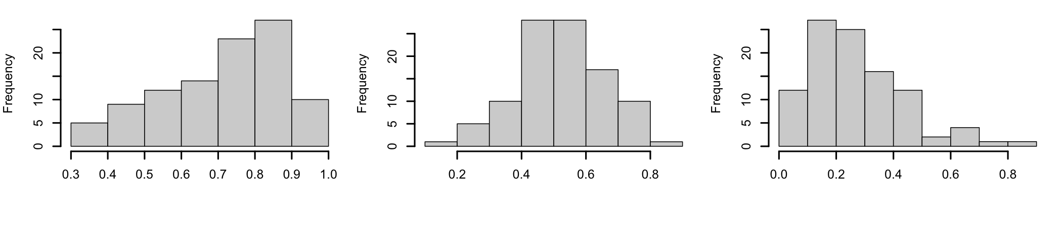
A more detailed interpretation (Bulmer 1979):
- Highly skewed if skewness < -1 or > +1;
- Moderately skewed, if skewness is between (-1 and -1/2) or between (+1/2 and +1);
- Approximately symmetric, if skewness is between -1/2 and +1/2.
8.1.3 Kurtosis
The normal distribution has a “balanced” shape, with tails that are neither too heavy nor too light. Kurtosis is a measure of how much the tails of the described distribution, that is, its extreme values, differ from those of the theoretical normal distribution44 Kurtosis is often described as the “peakedness” of a distribution, but it depends mostly on the tails. Two distributions with the same peak can have very different kurtosis.. The kurtosis of the normal distribution is 3. A value other than 3 means that extreme values are either more or less common than in the normal distribution. If the value is larger than 3, the distribution is called leptokurtic, with heavier tails, often with a sharper central peak: extreme values are more common than in a normal distribution. If the value is smaller than 3, the distribution is called platykurtic, with lighter tails, often with a flatter central peak: extreme values are less common than in a normal distribution.
4 Kurtosis is often described as the “peakedness” of a distribution, but it depends mostly on the tails. Two distributions with the same peak can have very different kurtosis.
Of note is the fact that statistical software does not always report the same number. Some programs report the kurtosis itself, which is 3 for the normal distribution. Others report the excess kurtosis, the kurtosis minus 3, which is 0 for the normal distribution. Before interpreting a value, check which of the two it is.
8.1.4 Testing Skewness and Kurtosis
The rules of thumb above ignore the size of the sample. A small sample can show a large skewness only by chance, while in a large sample even a small skewness is a reliable feature of the data. Skewness and kurtosis can be tested by dividing them by their standard errors, which depend only on the sample size55 The approximations \sqrt{6/n} and \sqrt{24/n} are often used for large samples.:
5 The approximations \sqrt{6/n} and \sqrt{24/n} are often used for large samples.
SE_{skewness} = \sqrt{\frac{6n(n - 1)}{(n - 2)(n + 1)(n + 3)}} \qquad SE_{kurtosis} = 2 SE_{skewness}\sqrt{\frac{n^2 - 1}{(n - 3)(n + 5)}}
The resulting z values, z = skewness / SE_{skewness} and z = (kurtosis - 3) / SE_{kurtosis}, are compared with the critical values of the standard normal distribution. A z value larger than 1.96 in absolute value indicates a significant departure from normality at \alpha = .05. In medium samples, a stricter threshold of 3.29 (\alpha = .001) is often used, and in large samples, of several hundred cases, the tests become too sensitive, and the size of the skewness and kurtosis themselves should be judged instead.
As an example, let’s look at three variables from the 40 students of Describing Data: the weekly hours of study, the weekly hours of paid work, and the final exam scores.
| Variable | Skewness | z | Kurtosis | z |
|---|---|---|---|---|
| Study hours | -0.01 | -0.03 | 2.96 | -0.05 |
| Paid work hours | 1.91 | 5.12 | 6.62 | 4.93 |
| Exam score | -0.25 | -0.67 | 2.42 | -0.79 |
With 40 students, the standard errors are 0.374 for the skewness and 0.733 for the kurtosis. The study hours and the exam scores have small skewness and kurtosis, and none of their z values is significant. The hours of paid work are a different story: a skewness of 1.91 (z = 5.12) and a kurtosis of 6.62 (z = 4.93) show a distribution with a long tail to the right and more extreme values than a normal distribution66 As expected from a variable where most students work a few hours or not at all, and a few work close to full time.. Tests that assume this variable is normally distributed, such as a t-Test with the hours of paid work as the DV, should not be used without a transformation77 See Normalization, Standardization, and Data Transformation. or a non-parametric alternative.
6 As expected from a variable where most students work a few hours or not at all, and a few work close to full time.
8.2 Tests of Normality
8.2.1 Visual Checks
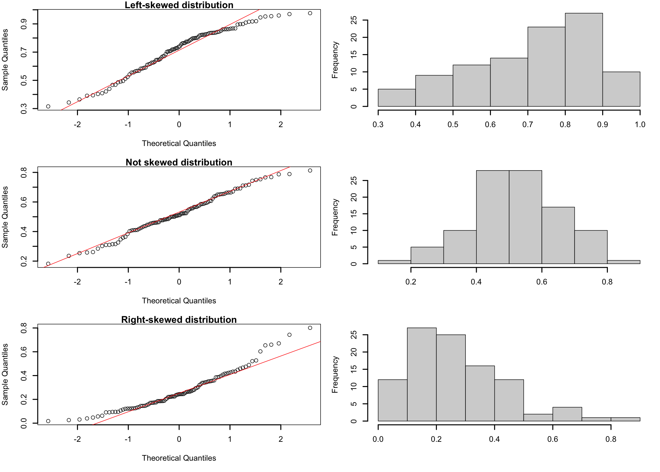
Visual checks can be used to assess, roughly, how close the sample’s distribution is to the normal distribution. This can be accomplished using Quantile-Quantile plots (qq-plots) that help visualize if a set of data comes from a theoretical distribution, the normal distribution in this case. In essence a qq-plot is just a scatter plot of two sets of quantiles, theoretical and observed, as they relate to each other88 Quantiles, also known as percentiles, are points in the data that divide the observations in intervals with equal probabilities. In essence, quantiles are just the data sorted in ascending order.. If the sample came from the desired distribution, the plot will roughly approximate a straight diagonal line. Any departure from that shape is an indication of departures from normality (Figure 8.3).
8 Quantiles, also known as percentiles, are points in the data that divide the observations in intervals with equal probabilities. In essence, quantiles are just the data sorted in ascending order.
Visually inspecting a qq-plot does not offer an exact and definitive proof that the sample data comes from a normal distribution. Nevertheless, it can be used to determine if further testing is necessary. For example, if the qq-plot has an S-shaped appearance, the sample data may be skewed.
8.2.2 More Specific Tests
Visual checks, while helpful, cannot be relied upon in most situations. Therefore, there are more specific tests that can be used to perform a more formal evaluation.
D’Agostino-Pearson omnibus test - Uses test statistics that combine skewness and kurtosis to compute a single p-value. This test has a tendency to hyper actively reject normality for small samples for which reason is not recommended to test normality of samples less than 20.
Kolmogorov-Smirnov test - Non-parametric test used to compare two samples that can serve as a goodness of fit test. When testing for normality for example, the sample data is standardized and compared with the theoretical normal distribution. It is less powerful than some other tests, such as Shapiro-Wilk.
Shapiro-Wilk’s W test - Tests the null hypothesis that the data in the sample is part of a normally distributed population. The test computes the value of the W statistic and a p-value probability. Considering the commonly accepted 0.05 value for p, any computed p-value greater than 0.05 indicates that the null hypothesis cannot be rejected: the test found no evidence of a departure from normality. This is not proof that the population is normal. In small samples the test can miss even a large departure, and in large samples it flags departures too small to matter, so it should be read together with the plots and the skewness and kurtosis. Does not work well for samples with many identical values.
Chi-square test of goodness-of-fit - Looks at a single categorical variable from a population and attempts to assess how close to or consistent with a hypothesized distribution the actual distribution of that varialbe is. See Goodness-of-Fit Test for more details.
8.3 Homogeneity of Variances or Homoscedasticity
The assumption of homogeneity of variances expects the variances in the different groups of the design to be identical. The homogeneity of variances is a standard assumption for many statistical tests and therefore it needs to be assessed so that the test results can be interpreted with confidence.
So, why is it important to test it? Many of the most common tests in statistical analysis99 For example, ANOVA assumes that observations are randomly selected from the population and that all observations come from the same population (or underlying group), with the same degree of variability, following the same distribution. are part of a category of tests called general linear models. These models are linear in the sense that they add things together. To be able to add things together, these tests assume that the distributions of the things being added are the same. Otherwise, if distributions are not the same, the results/estimate and the conclusion could be biased (usually overestimation of goodness of fit), therefore effectively rendering the test results unusable.
9 For example, ANOVA assumes that observations are randomly selected from the population and that all observations come from the same population (or underlying group), with the same degree of variability, following the same distribution.
In case of ANOVA, for example, if the variance of separate groups is significantly different, the p-values the test computes are no longer accurate because they are calculated based on the fact that certain results occur if the null hypothesis is true.
Let’s look at a few of the more common tests one can use to investigate the homogeneity of variances.
Bartlett test for homogeneity of variances - Tests the hypothesis (null hypothesis) that the variances in each sample groups are the same. This is the preferred test if the data is normally distributed, but it has a higher likelihood to produce false positive results when the data is non-normal. Therefore, Bartlett’s is preferred when the data comes from a known normal or close to normal distribution.
Levene’s test - A more robust inferential statistic alternative to the Bartlett test used to evaluate or assess the equality of variances for a variable that has two or more groups. If the computed p-value is less then the set significance level1010 E.g., the usual 0.05., the sample variance is unlikely due to random sampling from a population with equal variances. Therefore, the null hypothesis that the variances are the same is rejected. The Levene’s test is less sensitive to departures from normality than Bartlett’s.
10 E.g., the usual 0.05.
Fligner-Killeen test - Non-parametric test, robust for data sets with departures from normality. Can be useful if the normality of the sample data for groups is not observed.
8.4 Outliers
Outliers, extreme values data depart significantly from the majority of the values in the data set, can have substantial influence on the results of a statistical analysis. For example, they can skew the sample distribution to such extent that its departure from normality makes a large number of parametric statistical tests that require the data to be normal no longer applicable. Or, when present in many real-life time series data sets can significantly alter the outcomes of the analysis. For example, when analyzing an economic phenomenon, a hurricane affecting some link of the supply chain can produce a specific and significant change for a short period of time, which can influence the understanding of the phenomenon in average conditions.
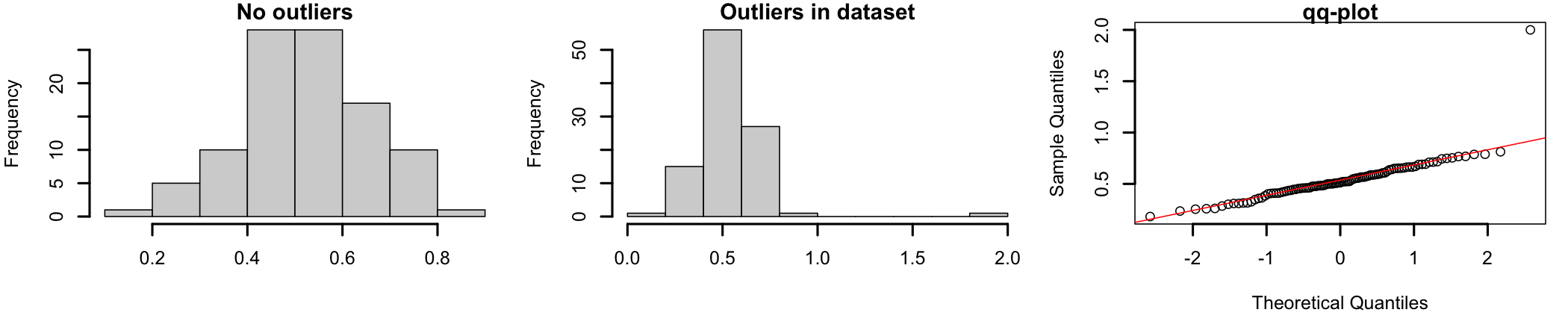
Figure 8.4 shows how outliers can influence the shape of the dataset’s distribution. The graph on the left shows a set of normally distributed data1111 The same data used previously in this section to discuss skewness. For this graph the data ranges between 0 and 1.. The graph in the middle represents the same data set to which two data points were added as outliers1212 For exemplification, one value, 2, was added to simulate a possible outlier. The point is located outside the range of the original dataset.. A visual inspection shows how the addition of the two outlying data points “pushes” the distribution to the left, away from the shape of normally distributed data. The qq-plot in the graph on the right shows how the two outliers influence dataset normality.
11 The same data used previously in this section to discuss skewness. For this graph the data ranges between 0 and 1.
12 For exemplification, one value, 2, was added to simulate a possible outlier. The point is located outside the range of the original dataset.
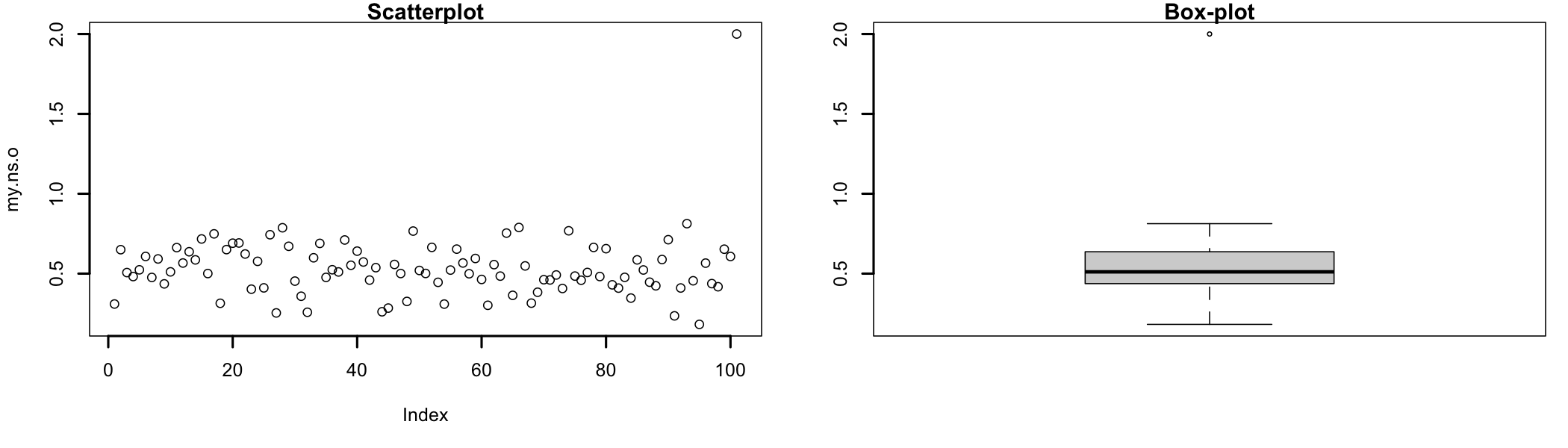
Most of the times outliers can be identified visually, in graphical representation such as scatterplots (Figure 8.5 left), box plots (Figure 8.5 right), or mahalanobis distances1313 The use of mahalanobis distance is better understood in context. See the outliers section in multiple regression.. In scatterplots outliers are represented as points plotted away from the “cloud” formed by majority of the data set. In box plots1414 Also known as box-and-whisker diagrams, are used to represent data graphically based on quartiles they would be indicated by individual points plotted on the graph. Mahalanobis distances1515 Mahalanobis distance (MD) is the distance between two points in multivariate space. It measures the distance relative to a base or central point considered as an overall mean for multivariate data (centroid). The centroid is a point in multivariate space where the means of all variables intersect., when represented as a histogram, will indicate the possible existence of an outliers by the presence of bars at the right side of the graph.
13 The use of mahalanobis distance is better understood in context. See the outliers section in multiple regression.
14 Also known as box-and-whisker diagrams, are used to represent data graphically based on quartiles
15 Mahalanobis distance (MD) is the distance between two points in multivariate space. It measures the distance relative to a base or central point considered as an overall mean for multivariate data (centroid). The centroid is a point in multivariate space where the means of all variables intersect.
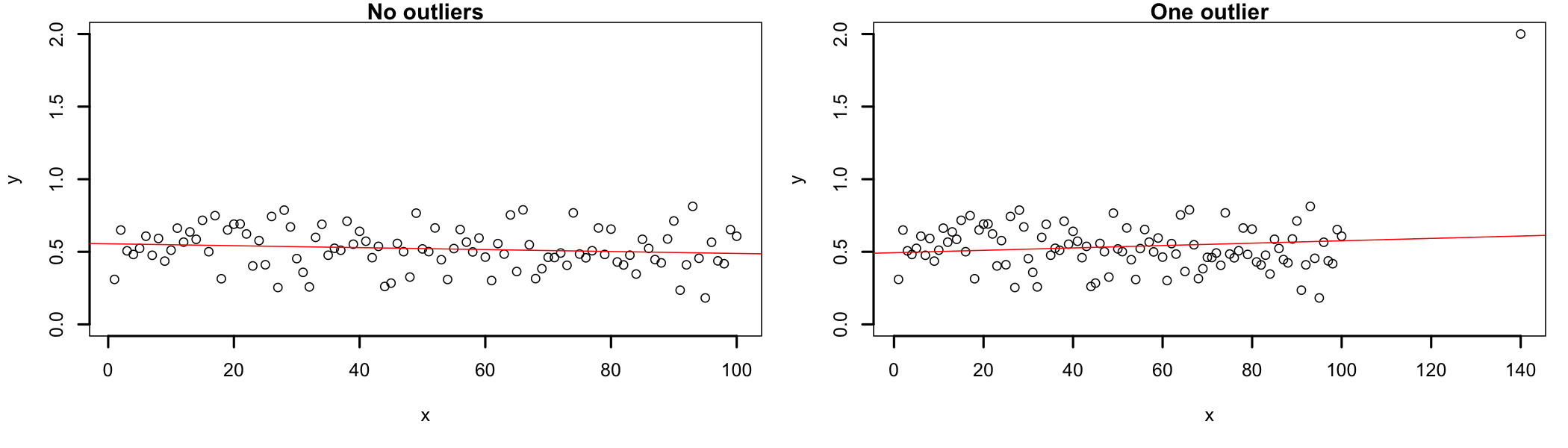
Linear regression presents itself as one of the better ways to explain how outliers can influence the outcomes of the analysis because these extreme values can substantially influence the slope of the regression line1616 This, in turn, will affect how well the regression equation will fit the data and the correlations coefficient. A single outlier can decrease the value of a correlation coefficient to the extent that the analysis rejects the existence of a real phenomenon.. In figure 8.6, the left side shows the data set without outliers and the right side shows the data set with one added outlier. Visually, the slope of the regression line (in red) changes from negative to positive when the outliers are not removed from the dataset. The change in slope may look small in the image below, but it could be significant in the analysis.
16 This, in turn, will affect how well the regression equation will fit the data and the correlations coefficient. A single outlier can decrease the value of a correlation coefficient to the extent that the analysis rejects the existence of a real phenomenon.
The way outliers are approached depends largely on the type of analysis being conducted and the type of data being analyzed. So far a widely accepted numerical method to deal with outliers does not seem to exist. Therefore, while in this resource approaches to outliers will be discussed when relevant to the statistical test and example, there are few guidelines that may be helpful across tests.
Outliers investigation is highly contextual and the criteria used for analysis ranges from theoretical necessity to common sense. There are legitimate situations when automatic (mathematical) removal of outliers makes sense. For example, when studying people reaction times to some stimulus and the vast majority of data points are in the milliseconds range, values in the seconds range most likely indicate distracted participants and therefore they could be safely removed. Alternatively, in situations where outliers consistently show up across groups, design cells, or successive measurement, they could indicate the existence of a different phenomenon than those under direct study. When their presence is detected, each outlier should be investigated individually and a decision made if it should be corrected1717 For example, in situations when the existence of an outlier is due to improper data input., removed1818 In cases when the data point is determined to be an aberrant measurement., or retained1919 When the outlier proves to be a true measurement and there are practical and/or theoretical reasons to be included in the analysis. in the analysis.
17 For example, in situations when the existence of an outlier is due to improper data input.
18 In cases when the data point is determined to be an aberrant measurement.
19 When the outlier proves to be a true measurement and there are practical and/or theoretical reasons to be included in the analysis.