18 Correlations
Correlations11 Remember, Correlation does not imply causation! explore how two or more variables are related to each other. It attempts to assess if the changes in one variable systematically vary with the changes in another. There is no dependence relationship between variables (e.g., IV/DV). Most often correlations are used to look at how variables are correlated to each other in a data set, usually with a focus on the variable(s) of interest.
1 Remember, Correlation does not imply causation!
This chapter explores the three most common correlation tests, one parametric (Pearson) and two non-parametric (Spearman and Kendall), followed by coefficients for special situations: when a third variable has to be taken into account, and when one of the variables is dichotomous. All three tests compute a correlation coefficient that can range between -1 and 1. The closer the value is to the extreme (-1 or 1) the stronger the relationship is.
- < 0 - indicates a negative correlation, meaning that the as the value of x increases, the value of y decreases.
- 0 - indicates no association.
- > 0 - indicates a positive correlation, meaning that as the value of x increases, the value of y increases as well.
The data set used in the examples below is called mtcars and is a classic example data set. The data, covering 11 variables describing cars, was extracted from the 1974 Motor Trend US magazine (Table 18.1).
| Variable | Description |
|---|---|
| mpg | Miles/gallon (US) |
| cyl | Number of cylinders |
| disp | Displacement (in cubic inches) |
| hp | Horsepower |
| drat | Rear axle ratio |
| wt | Weight (in 1000 lb) |
| qsec | 1/4 mile time |
| vs | Engine (0-V, 1-Line) |
| am | Transmission (0-automatic, 1-manual) |
| gear | Number of forward gears |
| carb | Number of carburators |
The first few rows of the data set are shown in Table 18.2.
| mpg | cyl | disp | hp | drat | wt | qsec | vs | am | gear | carb | |
|---|---|---|---|---|---|---|---|---|---|---|---|
| Mazda RX4 | 21.0 | 6 | 160 | 110 | 3.90 | 2.620 | 16.46 | 0 | 1 | 4 | 4 |
| Mazda RX4 Wag | 21.0 | 6 | 160 | 110 | 3.90 | 2.875 | 17.02 | 0 | 1 | 4 | 4 |
| Datsun 710 | 22.8 | 4 | 108 | 93 | 3.85 | 2.320 | 18.61 | 1 | 1 | 4 | 1 |
| Hornet 4 Drive | 21.4 | 6 | 258 | 110 | 3.08 | 3.215 | 19.44 | 1 | 0 | 3 | 1 |
| Hornet Sportabout | 18.7 | 8 | 360 | 175 | 3.15 | 3.440 | 17.02 | 0 | 0 | 3 | 2 |
| Valiant | 18.1 | 6 | 225 | 105 | 2.76 | 3.460 | 20.22 | 1 | 0 | 3 | 1 |
The question asked is: Is there any relationship between mpg and wt? That is, is there any correlation between the car’s weight and its fuel efficiency?
Hypotheses. All three tests below answer the same question:
- Null hypothesis (H0): In the population, there is no correlation between mpg and wt. The correlation coefficient (r, \varrho, or \tau, depending on the test) is zero.
- Alternative hypothesis (H1): In the population, mpg and wt are correlated. The correlation coefficient is not zero.
Decision criteria. The significance level is set before the analysis at \alpha = .05. The test is two-tailed, because the hypothesis does not predict whether the relationship is positive or negative. H0 is rejected if the p-value of the test is smaller than \alpha.
18.1 From Covariance to Correlation
Before running the tests, let’s see where the correlation coefficient comes from. Two variables are related when their values move together: when one is above its mean, the other tends to be above its mean as well (a positive relationship), or below it (a negative relationship). The covariance measures this tendency. For each case, the deviation of x from its mean is multiplied by the deviation of y from its mean. The product, called a cross-product, is positive when both deviations have the same sign and negative when they have opposite signs. The covariance is the sum of the cross-products divided by n - 1:
cov(x, y) = \frac{\sum(x_i - \bar{x})(y_i - \bar{y})}{n - 1}
For the weight (in 1000 lb) and the fuel efficiency (in miles per gallon) of the 32 cars, the covariance is -5.12. The negative sign shows that heavier cars tend to have lower fuel efficiency. The size of the covariance, however, is hard to interpret, because it depends on the units of the two variables22 Measuring the weight in pounds instead of thousands of pounds would multiply the covariance by 1,000, without changing the relationship.. Dividing it by the product of the two standard deviations removes the units and results in the correlation coefficient, which always lies between -1 and 1:
2 Measuring the weight in pounds instead of thousands of pounds would multiply the covariance by 1,000, without changing the relationship.
r = \frac{cov(x, y)}{s_x s_y} = \frac{-5.12}{0.98 \times 6.03} = -0.87
[1] -5.116685[1] -0.8676594The square of the correlation coefficient, the coefficient of determination (r^2), is the proportion of the variance the two variables share. Here, r^2 = 0.75: 75% of the differences in fuel efficiency between the cars are related to the differences in their weight, and the other 25% to other characteristics.
The significance of a correlation is tested with a t statistic with n - 2 degrees of freedom:
t = \frac{r\sqrt{n - 2}}{\sqrt{1 - r^2}} = \frac{-0.87\sqrt{30}}{\sqrt{1 - 0.75}} = -9.56
The test depends on the sample size as much as on the strength of the relationship33 The denominator, \sqrt{1 - r^2}, depends on the variance the two variables do not share.: with a large sample, even a weak correlation is significant. For this reason, the size of the coefficient, and not only its significance, should always be interpreted.
3 The denominator, \sqrt{1 - r^2}, depends on the variance the two variables do not share.
18.2 Pearson Correlations Test
At a glance
- Question
- Are two variables linearly related, and how strongly?
- Design
- Correlational, two variables measured on the same participants
- Variables
- Two, interval or ratio
- Assumptions
-
- Bivariate normal data
- A linear relationship
- No influential outliers
- Null hypothesis
- The population correlation is zero (\rho = 0)
- Test statistic
- r, tested with t and n - 2 degrees of freedom
- Effect size
- r itself: .10 small, .30 medium, .50 large; r2 is the shared variance
- If conditions fail
-
- The data is ordinal, not normal, or the relationship is monotonic but not linear → Spearman or Kendall correlation
- A third variable may explain the relationship → Partial correlation
- One variable is dichotomous → Point-biserial or biserial correlation
- Include in the write-up
-
- The number of participants
- r(df) = …, p = …, with its 95% CI
- The shared variance, r2
Parametric test used for two interval or ratio variables. The test requires the following assumptions to be met:
- Data is bi-variate normal;
- The relationship between variables is linear.
Before running the test, we verify the assumptions for the Pearson Correlations44 An issue with the Pearson correlations test is the fact that outliers can negatively impact the test results. Therefore, an analysis of outliers should be performed for the sample before the test. test.
4 An issue with the Pearson correlations test is the fact that outliers can negatively impact the test results. Therefore, an analysis of outliers should be performed for the sample before the test.
Bivariate normality means that the two variables are normally distributed together, and not only each on its own. It cannot be fully checked one variable at a time, but two variables that are not each normally distributed cannot be bivariate normal. The Shapiro-Wilk test of each variable is therefore a useful first check, together with the scatter plot below55 In a bivariate normal distribution, the points of the scatter plot form an elliptical cloud, denser in the middle, with no curves or separate clusters..
5 In a bivariate normal distribution, the points of the scatter plot form an elliptical cloud, denser in the middle, with no curves or separate clusters.
    Shapiro-Wilk normality test

data:  my.cor$mpg
W = 0.94756, p-value = 0.1229
    Shapiro-Wilk normality test

data:  my.cor$wt
W = 0.94326, p-value = 0.09265
The results show that neither variable departs significantly from the normal distribution (both p-values are > 0.05). Together with the scatter plot, there is no reason to doubt the assumption of normality.
Besides using Shapiro-Wilks, data normality can be analyzed using histograms, q-q plots, and the values of skewness and kurtosis for each data set. These alternative ways of studying a data set’s normality are exemplified for other analyses.
The linearity assumption can be visualized by generating a scatter plot representation with one variable on the X axis and the other variable on the Y axis.
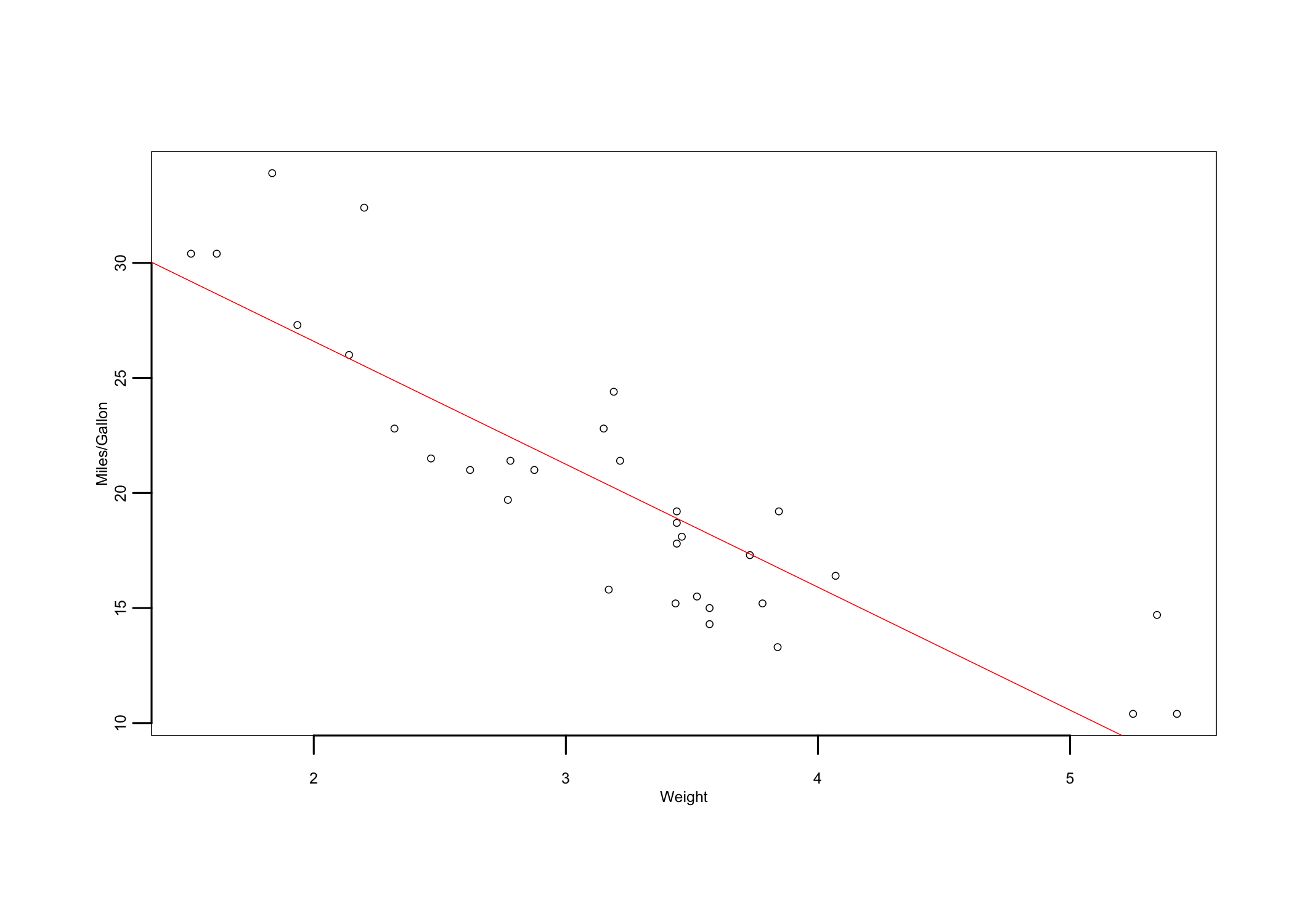
Looking at the scatter plot (Figure 18.1) the assumption of linearity seems to hold because the relationship between the two variables seems to be linear along the red line (regression line). Should the pattern of points show a different trend (e.g., curve), the relationship between the two variables is not linear and therefore other correlation tests should be used to analyze it.
With the assumptions verified, let’s run the Pearson Correlations test.
    Pearson's product-moment correlation

data:  my.cor$mpg and my.cor$wt
t = -9.559, df = 30, p-value = 1.294e-10
alternative hypothesis: true correlation is not equal to 0
95 percent confidence interval:
 -0.9338264 -0.7440872
sample estimates:
       cor
-0.8676594
Decision. With r = -0.87, p < .001, the p-value is smaller than \alpha = .05 and H0 is rejected: there is a significant correlation between mpg (fuel efficiency) and wt (car’s weight).
Effect size. The correlation coefficient is itself a measure of effect size. As a guide, absolute values around .10 indicate a small effect, around .30 a medium effect, and .50 or more a large effect. Here the effect is large and negative: heavier cars are less fuel efficient. Squaring the coefficient, r2 = 0.75, shows that weight accounts for about 75% of the variance in fuel efficiency.
18.3 Spearman Correlations Test
At a glance
- Use instead of
- The Pearson correlation, when the data is ordinal or not normal, or the relationship is monotonic but not linear
- Question
- Do two variables tend to increase or decrease together?
- Design
- Correlational, two variables measured on the same participants
- Variables
- Two, ordinal, interval, or ratio
- Assumptions
-
- Independent observations: each participant contributes one pair of values
- A monotonic relationship: as one variable increases, the other tends to increase, or to decrease, all along its range
- Null hypothesis
- The population rank correlation is zero
- Test statistic
- Spearman’s \varrho, the Pearson correlation of the ranks
- Effect size
- \varrho itself, read like r
- Include in the write-up
-
- The number of participants
- Why the rank-based coefficient was used
- \varrho = …, p = …
Non-parametric test used for two interval, ratio, or ordinal type variables.
The Spearman Correlations test does not assume that the data is normally distributed, because it works with the ranks of the values rather than with the values themselves. Besides independent observations, each participant contributing one pair of values, its only assumption concerns the shape of the relationship:
- Monotonic relationship: as one variable increases, the other tends to increase, or tends to decrease, all along its range, though not necessarily at a constant rate
- Detected using a scatter plot of the two variables;
- Violated when the relationship changes direction, such as a U-shaped curve66 A rank correlation, like Pearson’s r, can be close to zero for a strong relationship that changes direction..
6 A rank correlation, like Pearson’s r, can be close to zero for a strong relationship that changes direction.
The scatter plot used for the Pearson test (Figure 18.1) shows a relationship that decreases all along its range, so the test can be run directly.
    Spearman's rank correlation rho

data:  my.cor$mpg and my.cor$wt
S = 10292, p-value = 1.488e-11
alternative hypothesis: true rho is not equal to 0
sample estimates:
      rho
-0.886422
Decision. With \varrho = -0.89, p < .001, H0 is rejected: the two variables are significantly correlated to each other.
Effect size. The coefficient, \varrho = -0.89, indicates a large negative relationship, consistent with the Pearson result.
18.4 Kendall Correlations Test
At a glance
- Use instead of
- The Pearson correlation, like Spearman’s \varrho; often preferred with small samples or many tied ranks
- Question
- Do two variables tend to increase or decrease together?
- Design
- Correlational, two variables measured on the same participants
- Variables
- Two, ordinal, interval, or ratio
- Assumptions
-
- A monotonic relationship
- Null hypothesis
- The population \tau is zero
- Test statistic
- Kendall’s \tau, from the pairs of observations that agree or disagree in their order
- Effect size
- \tau, usually smaller than r or \varrho for the same data
- Include in the write-up
-
- The number of participants
- Why the rank-based coefficient was used
- \tau = …, p = …
Non-parametric test used for two interval, ratio, or ordinal type variables.
Like the Spearman test, the Kendall Correlations test works with the order of the values and assumes only a monotonic relationship between the two variables. Of note is the fact that Kendall’s \tau is often preferred to Spearman’s \varrho with small samples or with many tied ranks77 Tied ranks occur when several values are equal, which is common with ordinal data such as Likert items..
7 Tied ranks occur when several values are equal, which is common with ordinal data such as Likert items.
    Kendall's rank correlation tau

data:  my.cor$mpg and my.cor$wt
z = -5.7981, p-value = 6.706e-09
alternative hypothesis: true tau is not equal to 0
sample estimates:
       tau
-0.7278321
Decision. With \tau = -0.73, p < .001, H0 is rejected: the two variables are significantly correlated to each other.
Effect size. Kendall’s \tau is usually smaller than Pearson’s r or Spearman’s \varrho for the same data, because it is computed from pairs of observations rather than from the values or their ranks. A value of \tau = -0.73 still indicates a strong negative relationship.
18.5 Partial and Semi-Partial Correlations
At a glance
- Question
- Are two variables related once a third variable is taken into account?
- Design
- Correlational, three or more variables measured on the same participants
- Variables
- Interval or ratio
- Assumptions
-
- The assumptions of the Pearson correlation
- Linear relationships with the variable that is removed
- Null hypothesis
- The partial (or semi-partial) correlation is zero
- Test statistic
- Partial r, with n - 3 degrees of freedom for one removed variable
- Effect size
- The coefficient itself; the squared semi-partial correlation is the variance one variable explains on its own
- Include in the write-up
-
- The variable that was controlled
- Partial r(df) = …, p = …, next to the zero-order r
A correlation between two variables can be due, in part or entirely, to a third variable related to both. Heavier cars, for example, also tend to have more powerful engines (hp, horsepower), and more powerful engines use more fuel. Part of the correlation between weight and fuel efficiency may therefore be due to the engine. Two coefficients take a third variable into account:
- The partial correlation is the correlation between x and y after the third variable, z, has been removed from both of them. It answers the question: how are weight and fuel efficiency related among cars with the same horsepower?
- The semi-partial correlation (also called part correlation) is the correlation between y and x after z has been removed from x only. Its square is the proportion of the variance of y that x explains on its own, beyond what z already explains88 It is the basis of the contribution of each predictor in multiple regression..
8 It is the basis of the contribution of each predictor in multiple regression.
“Removing” a variable means using the residuals of a regression on it: the part of a variable that the third variable cannot predict. Let’s compute both coefficients this way:
[1] -0.7512049[1] -0.473654The correlation between weight and fuel efficiency was -0.87. Among cars with the same horsepower, it drops to -0.75, but remains strong and significant, t(29) = -6.13, p < .00199 A partial correlation is tested like a correlation, with one degree of freedom less for each variable removed.. The semi-partial correlation, -0.47, shows that the part of the weight not related to horsepower explains (-0.47)^2 = 0.22 of the variance of fuel efficiency on its own, 22%. Weight matters for fuel efficiency even when the engine is taken into account.
9 A partial correlation is tested like a correlation, with one degree of freedom less for each variable removed.
Of note is the fact that the partial correlation is always at least as large, in absolute value, as the semi-partial correlation. The partial correlation compares the unique part of x with what is left of y after z, while the semi-partial correlation compares it with all of y.
18.6 Point-Biserial and Biserial Correlations
At a glance
- Question
- How strongly is a continuous variable related to a dichotomous one?
- Design
- Correlational, or two groups compared on a continuous variable
- Variables
- One interval or ratio; one dichotomous
- Assumptions
-
- Point-biserial: the dichotomy is real (two truly distinct categories)
- Biserial: the dichotomy cuts a normally distributed continuous variable in two
- Null hypothesis
- The population correlation is zero
- Test statistic
- rpb, the Pearson correlation with the categories coded 0 and 1 (its test is the independent samples t-Test); or rb
- Effect size
- The coefficient itself, read like r
- Include in the write-up
-
- Which coefficient was used, and why
- rpb (or rb) = …, p = …
When one of the two variables is dichotomous, the correlation coefficient depends on what the dichotomy represents:
- The point-biserial correlation (r_{pb}) is used when the dichotomy is real, with two truly distinct categories, such as automatic and manual transmissions, or treatment and control groups. It is the Pearson correlation computed with the categories coded 0 and 1;
- The biserial correlation (r_{b}) is used when the dichotomy has been created by cutting a continuous variable in two, such as pass and fail on an exam scored from 0 to 100. It estimates the correlation with the underlying continuous variable, and assumes that this variable is normally distributed.
The type of transmission (am: 0 = automatic, 1 = manual) is a real dichotomy:
    Pearson's product-moment correlation

data:  my.cor$mpg and my.cor$am
t = 4.1061, df = 30, p-value = 0.000285
alternative hypothesis: true correlation is not equal to 0
95 percent confidence interval:
 0.3175583 0.7844520
sample estimates:
      cor
0.5998324
The point-biserial correlation, r_{pb} = 0.60, p < .001, shows that cars with a manual transmission have higher fuel efficiency. The test of r_{pb} is the independent samples t-Test: a t-Test comparing the fuel efficiency of the two kinds of transmission, with equal variances, gives the same t value and p-value.
For a biserial correlation, let’s return to the 40 students of Describing Data. Their exam scores were turned into a pass (60 points or more) or fail outcome, and the question is how the outcome is related to the weekly hours of study. The point-biserial correlation underestimates the relationship with the underlying exam score, because cutting a continuous variable in two discards information. The biserial correlation corrects it:
r_{b} = r_{pb}\frac{\sqrt{pq}}{h}
where p and q are the proportions of cases in the two categories and h is the height of the standard normal curve at the point that divides it in proportions p and q.
[1] 0.2884454[1] 0.3859929With 72% of the students passing, the point-biserial correlation, 0.29, becomes a biserial correlation of 0.391010 For comparison, the Pearson correlation between the hours of study and the exam score itself is 0.56.. Of note is the fact that the biserial correlation is only an estimate: when the original scores are available, they should be used.
10 For comparison, the Pearson correlation between the hours of study and the exam score itself is 0.56.
18.7 Bootstrapped Confidence Intervals
The confidence interval usually reported for a Pearson correlation assumes that the two variables are normally distributed. The Spearman and Kendall tests report no confidence interval at all. Bootstrapping provides an interval in both cases. It draws thousands of samples, with replacement, from the data, computes the coefficient in each of them, and uses the middle 95% of the values as the confidence interval.
BOOTSTRAP CONFIDENCE INTERVAL CALCULATIONS
Based on 5000 bootstrap replicates

CALL :
boot.ci(boot.out = my.boot, type = "perc")

Intervals :
Level     Percentile
95%   (-0.9472, -0.7463 )
Calculations and Intervals on Original Scale
The 95% bootstrap confidence interval of the Spearman correlation between fuel efficiency and weight runs from -0.95 to -0.75. It does not include zero, which confirms that the correlation is significant, and it shows that, even at its weakest, the relationship is strong. With only 32 cars, the interval is fairly wide1111 The bootstrap results change slightly every time the analysis is run, unless the random seed is fixed..
11 The bootstrap results change slightly every time the analysis is run, unless the random seed is fixed.
18.8 Reporting Correlations
When a study has several variables, their correlations are reported in a table, usually together with the means and the standard deviations of the variables (Table 18.3). Each correlation appears only once, below the diagonal.
| Variable | M | SD | 1 | 2 | 3 |
|---|---|---|---|---|---|
| 1. Fuel efficiency (mpg) | 20.09 | 6.03 | |||
| 2. Weight (1000 lb) | 3.22 | 0.98 | -.87*** | ||
| 3. Horsepower | 146.69 | 68.56 | -.78*** | .66*** | |
| 4. 1/4 mile time (s) | 17.85 | 1.79 | .42* | -.17 | -.71*** |
| Note. * p < .05. ** p < .01. *** p < .001. |
Here is an example of how to write up a correlation in a publication1212 The correlation coefficient is reported without a leading zero, because it cannot be larger than 1, and its degrees of freedom, n - 2, are given in parentheses.:
12 The correlation coefficient is reported without a leading zero, because it cannot be larger than 1, and its degrees of freedom, n - 2, are given in parentheses.
A Pearson correlation showed a strong negative relationship between the weight of 32 cars and their fuel efficiency, r(30) = -.87, p < .001, 95% CI [-.93, -.74]. Weight accounted for 75% of the variance in fuel efficiency. The relationship remained strong when horsepower was controlled, partial r(29) = -.75, p < .001.
18.9 Summary
The correlation coefficient is a standardized covariance: it measures how two variables move together, on a scale from -1 to 1 that does not depend on their units. Its square shows the proportion of variance the two variables share. The Pearson coefficient is used for interval and ratio data with a linear relationship, and the Spearman and Kendall coefficients for ordinal data or when the assumptions of the Pearson test are not met. Partial and semi-partial correlations take a third variable into account, the point-biserial and biserial correlations deal with dichotomous variables, and bootstrapping provides confidence intervals when the usual formulas do not apply.
Of note is the fact that a correlation, however strong, does not show which variable affects the other, or whether either does. In the example, it is reasonable to believe that the weight of a car affects its fuel efficiency, but the data alone cannot prove it, and the partial correlations showed that part of the relationship is due to other characteristics of the cars1313 See A Few Words About Causality..
13 See A Few Words About Causality.