20 Simple Linear Regression
At a glance
- Question
- Does one variable predict another, and by how much?
- Design
- Correlational or experimental, two variables measured on the same participants
- Criterion
- Interval or ratio
- Predictor
- Interval or ratio
- Assumptions
-
- A linear relationship between the predictor and the criterion
- Independent observations
- Normally distributed residuals (the variables themselves need not be)
- Homoscedasticity: residuals with constant variance
- Null hypothesis
- The slope is zero
- Test statistic
- t for the slope; F for the model (the same test with one predictor)
- Effect size
- R2, the variance explained; the standardized slope, \beta
- If conditions fail
-
- There are several predictors → Multiple linear regression
- The criterion is dichotomous → Logistic regression
- Include in the write-up
-
- The assumption checks
- b = …, SE = …, \beta = …, t(df) = …, p = …
- What the slope means in the units of the variables
- R2 and F(df1, df2) = …, p = …
Used to study/describe the predictive relationship between one criterion (DV) variable and one predictor (IV) variable, both measured on an interval or ratio scale. While correlations (see Correlations) look at how two variables vary together, with no dependence relationship between them, regression assumes a direction, from the predictor to the criterion. In addition, it provides an equation that can be used to predict the values of the criterion variable from the values of the predictor11 For example, predicting a student’s exam score from the number of hours they studied, or a car’s fuel efficiency from its weight..
1 For example, predicting a student’s exam score from the number of hours they studied, or a car’s fuel efficiency from its weight.
With two or more predictors, the analysis becomes a multiple linear regression. When the criterion has only two values, such as passing or failing a course, a logistic regression is used instead.
Simple linear regression is the building block of the more complex regression models. Multiple Linear Regression, for example, extends the same ideas to two or more predictors. For this reason, it is worth taking the time to understand how the simple model works before moving on to the more complex ones.
20.1 The Theory
20.1.1 The Model
The intent of the linear regression analysis is to find the line that best fits a set of data points. Each observed value of the criterion variable (Y_i) is described as a straight line plus an error:
Y_i = a + bX_i + e_i
In this equation a is the intercept22 The value of Y when X = 0, or the point where the line intersects the Y (vertical) axis., b is the slope of the line33 The change in Y for each one-unit change in X., and e_i is the error, also called the residual. The residual is the part of Y_i the line cannot explain. When the equation is used to predict values, the error is left out and the result is the predicted value \hat{Y}_i44 Read “Y-hat”. The notation is used to differentiate the predicted values from the observed values of Y.:
2 The value of Y when X = 0, or the point where the line intersects the Y (vertical) axis.
3 The change in Y for each one-unit change in X.
4 Read “Y-hat”. The notation is used to differentiate the predicted values from the observed values of Y.
\hat{Y}_i = a + bX_i \qquad e_i = Y_i - \hat{Y}_i
Of note is the fact that the values of a and b computed from the sample are only estimates of the population values, usually represented by \alpha and \beta.
20.1.2 The Line of Best Fit
There are many lines that can be drawn through a cloud of data points. The ordinary least squares (OLS) method chooses the line that makes the sum of the squared residuals as small as possible55 The residuals are squared so that the points above the line (positive residuals) and those below the line (negative residuals) do not cancel each other out.. Skipping the calculus, the slope and the intercept of this line are:
5 The residuals are squared so that the points above the line (positive residuals) and those below the line (negative residuals) do not cancel each other out.
b = \frac{cov(X, Y)}{var(X)} = r\frac{s_{Y}}{s_{X}} \qquad a = \bar{Y} - b\bar{X}
The second form of the slope equation shows the connection with the correlation coefficient r: the slope is the correlation rescaled from standard deviations to the units in which the two variables are measured. For the same reason, the slope is not a measure of effect size. Its value depends on the units of measurement66 A slope of 2 points per hour describes exactly the same relationship as a slope of 2/60 points per minute. and, on its own, says nothing about the strength of the relationship. Also, the least squares line always passes through the point defined by the two means (\bar{X}, \bar{Y}), and its residuals always add up to zero.
6 A slope of 2 points per hour describes exactly the same relationship as a slope of 2/60 points per minute.
20.1.3 How Well the Line Fits
Without a predictor, the best guess for any value of Y is its mean, \bar{Y}. The goodness of fit of the regression line is therefore assessed by comparing it with this basic model: how much better does the line predict than the mean? To answer this question we need three sums of squares (SS):
- Total sum of squares (SS_{T}), the sum of the squared differences between the observed values and the mean, \sum(Y_i - \bar{Y})^2. It represents the total variability in the data, the variability there is to explain;
- Residual sum of squares (SS_{R}), the sum of the squared differences between the observed values and the regression line, \sum(Y_i - \hat{Y}_i)^2. It represents the variability the model is not able to explain;
- Model sum of squares (SS_{M}), the difference between the two, SS_{M} = SS_{T} - SS_{R}. It represents the improvement in prediction brought by the regression line over the mean.
The coefficient of determination (R^2) is the proportion of the total variability explained by the model77 Multiplying R^2 by 100 gives the percentage of variance explained.:
7 Multiplying R^2 by 100 gives the percentage of variance explained.
R^2 = \frac{SS_{M}}{SS_{T}}
With only one predictor, R^2 is equal to the square of the correlation coefficient (r^2), and it is the effect size of the simple regression. Following Cohen’s guidelines for the correlation coefficient (.10, .30, and .50) (Cohen 1977), values around .01 indicate a small effect, .09 a medium effect, and .25 or more a large effect.
20.1.4 Testing the Model and the Predictor
The significance of the model is tested with an F ratio, the variability explained by the model divided by the variability left unexplained. Before computing the ratio, each sum of squares is divided by its degrees of freedom, resulting in the mean squares (MS):
F = \frac{MS_{M}}{MS_{R}} = \frac{SS_{M} / 1}{SS_{R} / (n - 2)}
With one predictor, the model has one degree of freedom and the residuals have n - 288 Two degrees of freedom are lost because two values, a and b, are estimated from the data..
8 Two degrees of freedom are lost because two values, a and b, are estimated from the data.
The significance of the predictor is tested with a t statistic, the slope divided by its standard error (s_{b}):
t = \frac{b}{s_{b}}
In both cases the null hypothesis states that, in the population, the slope is zero. That is, the regression line is flat and knowing the value of X does not help predict the value of Y. In the case of simple linear regression the two tests answer the same question. They produce the same p-value and F = t^2. This is no longer the case for Multiple Linear Regression, where the F test looks at all predictors together while each t test looks at only one of them.
20.1.5 The Standardized Slope
If both variables are first converted to z-scores (see Normalization), the regression line passes through the origin, the intercept is no longer needed99 The means of both variables are zero., and the slope becomes the standardized slope \beta^{*}, also known as the beta weight:
9 The means of both variables are zero.
z_{\hat{Y}} = \beta^{*} z_{X}
The standardized slope shows by how many standard deviations Y changes for each standard deviation change in X. In the case of simple linear regression it is equal to the correlation coefficient, r.
20.2 Assumptions
In regression analysis the assumptions are intertwined with the analysis itself. With the exception of linearity, which can be observed in a scatter plot of the data, the assumptions refer to the residuals and can only be verified after the model has been computed. Simple linear regression assumptions are:
- Linear relationship between the predictor (IV) and the criterion (DV) variables
- Detected using a scatter plot of the data and a plot of the residuals against the predicted values;
- Violated when the points follow a curve instead of a straight line.
- Independence of observations
- Usually ensured by the design of the study1010 E.g., each participant is measured only once and independently of the other participants.;
10 E.g., each participant is measured only once and independently of the other participants.
- Violated when the residuals form clusters or follow a pattern in time.
- Usually ensured by the design of the study1010 E.g., each participant is measured only once and independently of the other participants.;
- Normal distribution of residuals1111 The two variables themselves do not need to be normally distributed.
11 The two variables themselves do not need to be normally distributed.
- Detected using normal probability (q-q) plots of the residuals and tests of normality;
- Violated when the residuals fall far from the straight line of the plot.
- Homoscedasticity, residuals have constant variance
- Detected using a plot of the residuals against the predicted values and a test of non-constant variance;
- Violated when the spread of the residuals increases or decreases along the regression line1212 A pattern often described as a funnel shape. This situation is called heteroscedasticity..
12 A pattern often described as a funnel shape. This situation is called heteroscedasticity.
20.3 The Study
The one-sample t-Test showed that the 40 students enrolled in a three-credit course studied, on average, less than the 12 hours per week recommended by their university. At the end of the semester the same students took the final exam of the course, scored from 0 to 100. The question asked is: Do students who study more get higher scores on the exam? And, if they do, by how much? The data set1313 Column labels are: student, hours, and exam. was made up for this example. The first few rows of the data set are shown in Table 20.1.
13 Column labels are: student, hours, and exam.
| Student | Study hours | Exam score |
|---|---|---|
| 1 | 9.7 | 92 |
| 2 | 6.8 | 70 |
| 3 | 13.1 | 79 |
| 4 | 10.7 | 67 |
| 5 | 4.6 | 57 |
| 6 | 5.3 | 45 |
Hypotheses. The analysis below models the exam score (exam) as a function of the weekly study time (hours).
- Null hypothesis (H0): In the population, study time does not predict the exam score. The regression slope is zero (\beta = 0).
- Alternative hypothesis (H1): In the population, study time predicts the exam score. The regression slope is different from zero (\beta \neq 0).
Decision criteria. The significance level is set at \alpha = .05, and the test is two-tailed. The residuals have 40 - 2 = 38 degrees of freedom. H0 is rejected if the p-value of the slope is smaller than \alpha. The effect size is R^2.
As always, it is helpful to familiarize ourselves with the data before the analysis. Let’s take a look at some summary statistics.
     hours             exam
 Min.   : 3.300   Min.   :37.00
 1st Qu.: 9.025   1st Qu.:58.50
 Median :10.600   Median :70.00
 Mean   :10.703   Mean   :68.12
 3rd Qu.:13.100   3rd Qu.:77.25
 Max.   :19.000   Max.   :92.00
20.3.1 Linearity
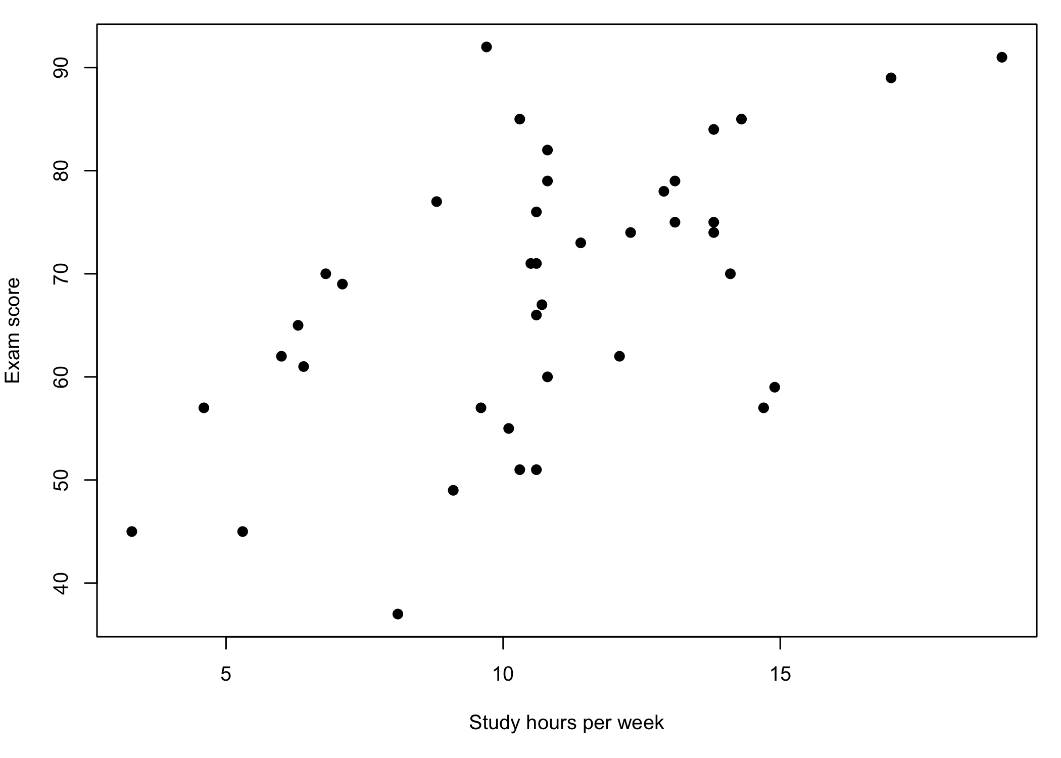
The scatter plot (Figure 20.1) shows the data points rising from left to right with no sign of a curve, which suggests a positive linear relationship between the two variables. The relationship is far from perfect, though. Students who studied about the same number of hours obtained quite different scores on the exam.
20.3.2 Fitting the Line
Using the means, the standard deviations, and the correlation coefficient (r = 0.56), let’s first compute the slope and the intercept by hand:
b = r\frac{s_{Y}}{s_{X}} = 0.56 \times \frac{13.45}{3.37} = 2.22
a = \bar{Y} - b\bar{X} = 68.12 - 2.22 \times 10.70 = 44.34
R finds the same values when it fits the model:
Call:
lm(formula = exam ~ hours, data = se)

Coefficients:
(Intercept)        hours
     44.341        2.222
Therefore, the regression equation is:
\widehat{exam} = 44.34 + 2.22 \times hours
The slope tells us that, for each additional hour of study per week, the exam score increases on average by about 2.2 points. The intercept is the predicted score of a student who does not study at all. Because none of the students in the sample studied less than 3.3 hours a week, the intercept is needed to position the line, but it does not describe an actual student1414 In general, the intercept should be interpreted with care when X = 0 is outside the range of the data, or is not a meaningful value..
14 In general, the intercept should be interpreted with care when X = 0 is outside the range of the data, or is not a meaningful value.
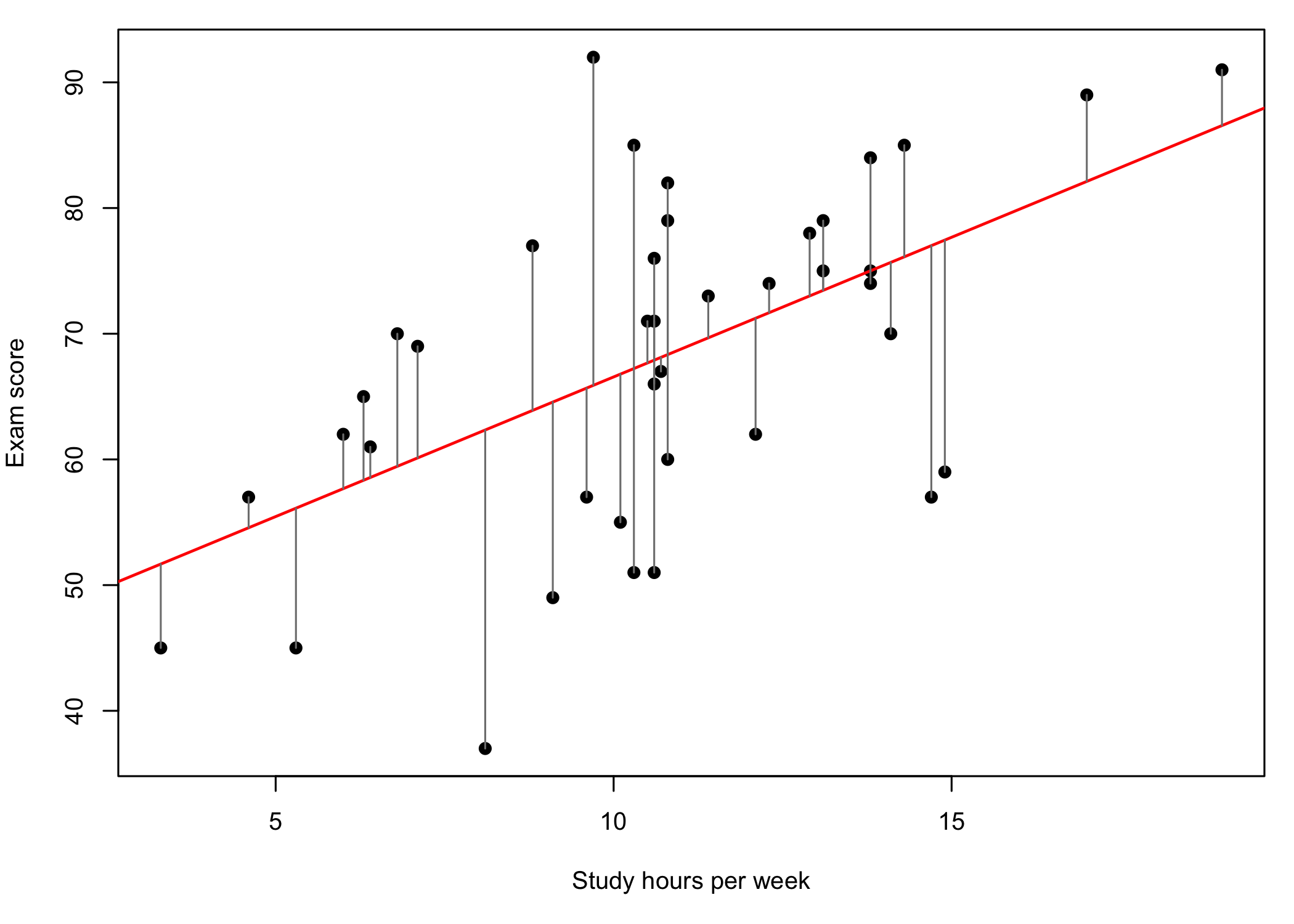
The grey segments in Figure 20.2 represent the residuals, the vertical distances between the observed exam scores and the regression line (red). The least squares method positions the line so that the sum of the squares of these distances is the smallest possible.
20.3.3 Checking the Assumptions
The independence of observations is supported by the design of the study: each student studied and took the exam on their own. The remaining assumptions are checked on the residuals.
    Shapiro-Wilk normality test

data:  resid(my.lm)
W = 0.97259, p-value = 0.433
Non-constant Variance Score Test
Variance formula: ~ fitted.values
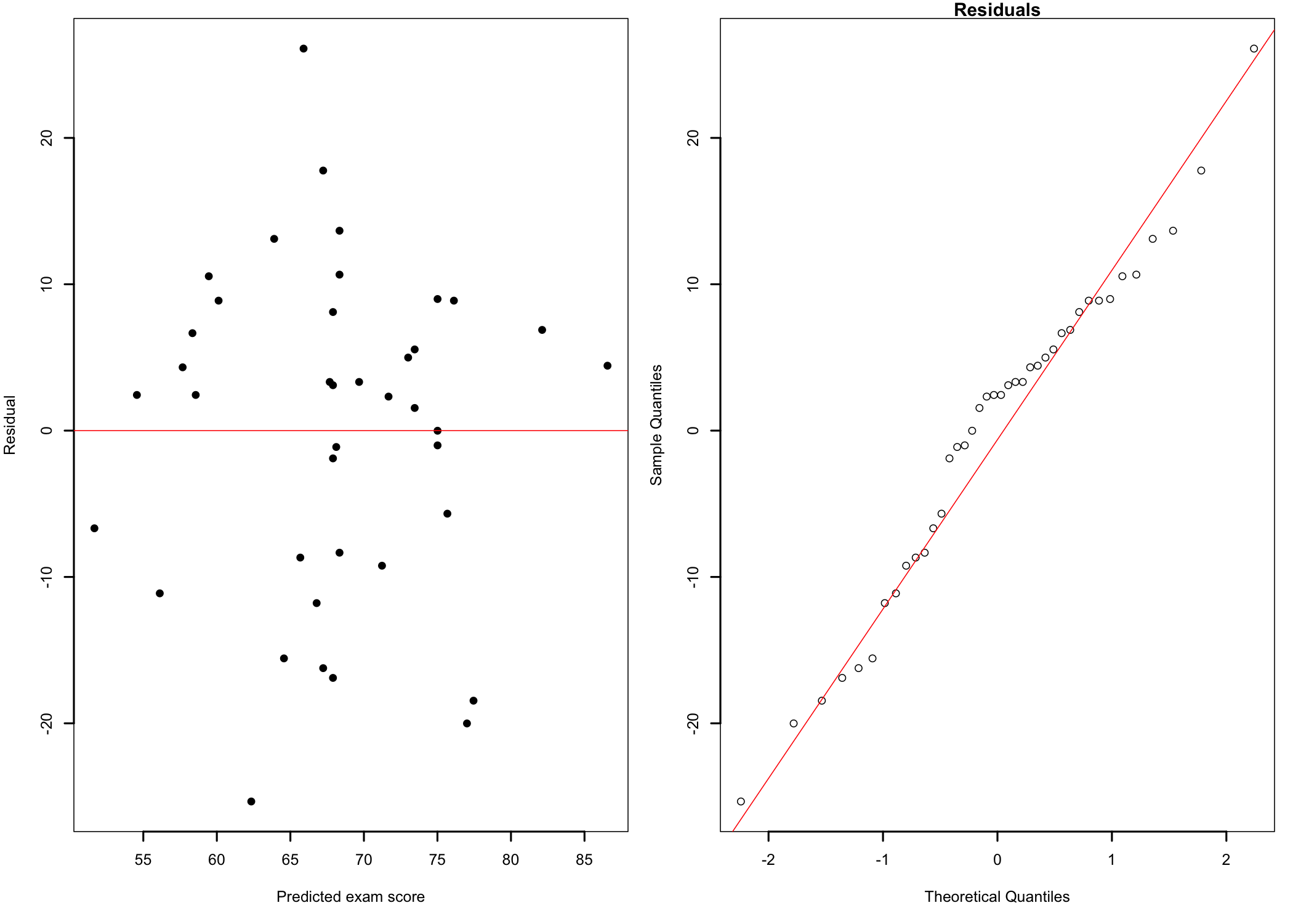
Chisquare = 0.09669521, Df = 1, p = 0.75583- Linearity and homoscedasticity. The residuals vs. predicted values plot (Figure 20.3 left) shows a homogeneous cloud of points around the zero line, with no curve and no funnel shape. The non-constant variance test1515 Also known as the Breusch-Pagan test. supports the same conclusion (p = .756). The null hypothesis that the variance of the residuals is constant cannot be rejected.
15 Also known as the Breusch-Pagan test.
- Normality of residuals. The grouping of the points close to the straight line of the q-q plot (Figure 20.3 right) shows no clear departure of the residuals from a normal distribution, and neither does the Shapiro-Wilk test (p = .433).
All assumptions are met, so we can proceed with the analysis.
20.3.4 The Model
Call:
lm(formula = exam ~ hours, data = se)

Residuals:
    Min      1Q  Median      3Q     Max
-25.341  -8.425   2.436   7.186  26.103

Coefficients:
            Estimate Std. Error t value Pr(>|t|)
(Intercept)  44.3411     6.0345   7.348 8.36e-09 ***
hours         2.2223     0.5385   4.127 0.000193 ***
---
Signif. codes:  0 '***' 0.001 '**' 0.01 '*' 0.05 '.' 0.1 ' ' 1

Residual standard error: 11.32 on 38 degrees of freedom
Multiple R-squared:  0.3095,    Adjusted R-squared:  0.2913
F-statistic: 17.03 on 1 and 38 DF,  p-value: 0.0001933
The output above has three parts:
- Coefficients, listing for the intercept and for the slope (the
hoursrow) the estimated value, its standard error, the t statistic1616 The estimated value divided by its standard error., and the p-value of the t statistic. Thehoursrow is the test of the predictor;16 The estimated value divided by its standard error.
- Residual standard error, 11.32 points, the typical distance between the observed exam scores and the regression line, on 38 degrees of freedom;
- R-squared and the F-statistic, the goodness of fit of the model and its test of significance.
The sums of squares used to compute R^2 and F can be found in the analysis of variance table of the model:
Analysis of Variance Table

Response: exam
          Df Sum Sq Mean Sq F value    Pr(>F)
hours      1 2183.4 2183.35  17.033 0.0001933 ***
Residuals 38 4871.0  128.18
---
Signif. codes:  0 '***' 0.001 '**' 0.01 '*' 0.05 '.' 0.1 ' ' 1
With SS_{M} = 2183.4 and SS_{R} = 4871.0, the total sum of squares is SS_{T} = 7054.4. Therefore:
R^2 = \frac{SS_{M}}{SS_{T}} = \frac{2183.4}{7054.4} = 0.310 \qquad F = \frac{2183.4 / 1}{4871.0 / 38} = 17.03
Decision. For the slope, t(38) = 4.13, p < .001. The p-value is smaller than \alpha = .05. The null hypothesis is rejected and the alternative hypothesis accepted: study time is a significant predictor of the exam score. The test of the model leads to the same conclusion, F(1, 38) = 17.03, p < .001. As expected, F is the square of t (4.132 = 17.03).
Effect size. R^2 = 0.31 indicates that study time accounts for about 31% of the variance of the exam scores, a large effect. The remaining 69% is due to other factors not included in the model1717 E.g., the students’ prior knowledge of the subject, their motivation, or how efficiently they studied.. The adjusted R^2 (0.29) corrects R^2 for the number of predictors in the model and becomes more relevant when there are several predictors.
17 E.g., the students’ prior knowledge of the subject, their motivation, or how efficiently they studied.
The standardized slope, \beta^{*} = 0.56, is equal to the correlation coefficient. An increase of one standard deviation in study time is associated with an increase of 0.56 standard deviations in the exam score.
20.3.5 Predicting New Values
The regression equation can now be used to predict the exam score of a student based on their study time. As an example, let’s predict the score of a student who studies the recommended 12 hours per week:
      fit      lwr      upr
1 71.0084 67.11822 74.89857
fit lwr upr
1 71.0084 47.76067 94.25612The predicted score is 44.34 + 2.22 \times 12 = 71.0 points. The output shows two intervals for the prediction, which answer two different questions:
- The confidence interval (67.1 to 74.9) is the interval for the mean score of all students who study 12 hours per week;
- The prediction interval (47.8 to 94.3) is the interval for the score of one student who studies 12 hours per week. It is much wider because individual scores vary around the mean.
Remember, predictions can be trusted only within the range of the data used to build the model, in this case between 3.3 and 19 hours per week. There is nothing in the data to suggest that the relationship stays the same outside this range. For example, the model would predict a score over 100 points for a student who studies 40 hours per week, which is not possible.
20.3.6 Reporting the Results
Finally, here is an example of how to write up the results in a publication.
A simple linear regression tested whether weekly study time predicted the final exam scores of 40 students. The relationship was linear, and the residuals did not depart significantly from normality (Shapiro-Wilk p = .433) with constant variance (p = .756). Study time significantly predicted exam scores, b = 2.22, SE = 0.54, β = .56, t(38) = 4.13, p < .001. Each additional hour of study a week was associated with an increase of 2.22 points in the exam score. The model explained 31% of the variance in exam scores, R2 = .31, F(1, 38) = 17.03, p < .001.
20.4 Summary
The analysis shows that the students who study more tend to get higher scores on the final exam, and that study time alone explains close to a third of the variability of the scores. Study time is, however, only one of the factors that contribute to the students’ performance. Adding other predictors to the model, such as prior knowledge or motivation, would require a multiple linear regression analysis.
Of note is the fact that, as with any regression on observational data, the results show that study time and exam scores vary together, not that studying more causes higher scores. Students who study more may also differ in other ways that affect their scores1818 For example, they may be more motivated or more interested in the subject. See A Few Words About Causality..
18 For example, they may be more motivated or more interested in the subject. See A Few Words About Causality.