7 Describing Data
Used to summarize and present the data collected in a study, descriptive statistics reduce a large number of values to a few numbers, tables, and graphs that are easy to read and to communicate. They describe only the sample at hand. Unlike the inferential statistics discussed in the following chapters, they make no claims about the population the sample was drawn from11 See Descriptive vs. Inferential Designs..
Describing the data is always the first step of an analysis, even when the purpose of the study is inferential. It shows what the data looks like, whether there are errors or unusual values in it, and whether the assumptions of the tests we intend to use are likely to be met. The statistics used to describe a variable depend on its scale of measurement22 See Measurement Scales.. Counts and percentages are used for categorical (nominal and ordinal) variables, while the mean, the median, and the standard deviation are used for numerical (interval and ratio) variables.
2 See Measurement Scales.
Three questions guide the description of a variable:
- How often does each value occur? Answered by the frequencies;
- What is a typical value? Answered by the measures of central tendency: the mean, the median, and the mode;
- How spread out are the values? Answered by the measures of variability: the range, the interquartile range, the variance, and the standard deviation.
7.1 The Study
The 40 students enrolled in the three-credit course we will meet again in the one-sample t-Test and in Simple Linear Regression were asked to fill in a short survey at the beginning of the semester. They reported their year of study, the program they are enrolled in, the number of hours they work at a paid job in a typical week, and how useful they expect the course to be for their future work33 On a five-point scale, from 1 = not at all useful to 5 = very useful.. Later in the semester, they reported the number of hours per week they studied for the course and, at the end of it, took the final exam. Before asking any questions about the students, let’s find out who they are. The data set44 Column labels are: student, year, program, work, hours, exam, and useful. was made up for this example. The first few rows of the data set are shown in Table 7.1.
3 On a five-point scale, from 1 = not at all useful to 5 = very useful.
4 Column labels are: student, year, program, work, hours, exam, and useful.
| Student | Year | Program | Work | Study hours | Exam score | Useful |
|---|---|---|---|---|---|---|
| 1 | Sophomore | Education | 0 | 9.7 | 92 | 3 |
| 2 | First-year | Education | 6 | 6.8 | 70 | 3 |
| 3 | Sophomore | Psychology | 0 | 13.1 | 79 | 4 |
| 4 | Sophomore | Education | 22 | 10.7 | 67 | 2 |
| 5 | Sophomore | Psychology | 2 | 4.6 | 57 | 5 |
| 6 | Sophomore | Business | 0 | 5.3 | 45 | 4 |
The variables and their scales of measurement are:
- year, the year of study, ordinal55 The categories have a natural order, from first-year to senior, but the distance between two consecutive years has no meaning for this study.;
5 The categories have a natural order, from first-year to senior, but the distance between two consecutive years has no meaning for this study.
- program, the program of study, nominal;
- work, the hours of paid work per week, ratio;
- hours, the hours of study per week, ratio;
- exam, the final exam score, from 0 to 100, ratio66 As a count of points, the score has a true zero. As a measure of what the students know, it is closer to an interval scale: a score of 0 does not mean no knowledge, and 80 does not mean twice the knowledge of 40.;
6 As a count of points, the score has a true zero. As a measure of what the students know, it is closer to an interval scale: a score of 0 does not mean no knowledge, and 80 does not mean twice the knowledge of 40.
- useful, the expected usefulness of the course, ordinal77 A single rating item is ordinal. The distance between “not at all useful” (1) and “slightly useful” (2) is not necessarily the same as the distance between “useful” (4) and “very useful” (5)..
7 A single rating item is ordinal. The distance between “not at all useful” (1) and “slightly useful” (2) is not necessarily the same as the distance between “useful” (4) and “very useful” (5).
7.2 Frequencies
Used with categorical data, the frequencies show how many times each category occurs in the data set. On their own, counts are hard to compare across groups or studies of different sizes, so they are usually reported together with:
- the relative frequency, the count divided by the total number of cases, a proportion between 0 and 1;
- the percentage, the relative frequency multiplied by 100;
- the cumulative percentage, the percentage of cases at or below a given category. It is meaningful only for ordinal variables88 For a nominal variable, such as the program, the order of the categories is arbitrary and so is any running total., where the categories have a natural order.
8 For a nominal variable, such as the program, the order of the categories is arbitrary and so is any running total.
| Program | n | % |
|---|---|---|
| Psychology | 14 | 35.0 |
| Nursing | 13 | 32.5 |
| Education | 9 | 22.5 |
| Business | 4 | 10.0 |
| Year | n | % | Cumulative % |
|---|---|---|---|
| First-year | 5 | 12.5 | 12.5 |
| Sophomore | 23 | 57.5 | 70.0 |
| Junior | 7 | 17.5 | 87.5 |
| Senior | 5 | 12.5 | 100.0 |
Table 7.2 shows that most of the students come from Psychology (35.0%) and Nursing (32.5%), and only 4 from Business. The program is a nominal variable, so the rows were ordered from the largest to the smallest group, which makes the table easier to read. The year of study (Table 7.3) is ordinal, so its categories keep their natural order. More than half of the students are sophomores, and the cumulative percentage shows that 70.0% of them are in their first or second year.
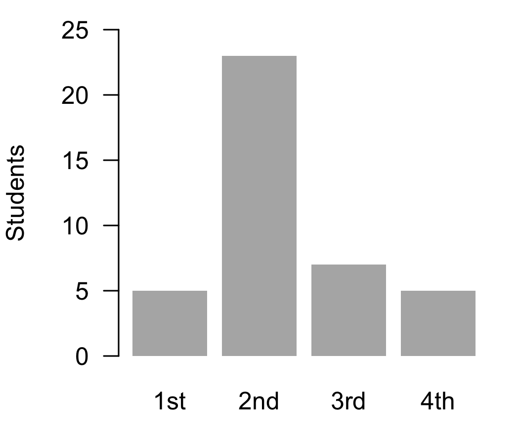
The same information can be shown in a bar chart (Figure 7.1), with one bar for each category and the height of the bar showing the count or the percentage. The bars are separated by gaps, a reminder that the categories are distinct99 In a histogram, which shows numerical data, the bars touch, because the values are continuous.. Pie charts are also common, but the angles of the slices are harder to compare than the heights of the bars, especially when there are more than a few categories.
9 In a histogram, which shows numerical data, the bars touch, because the values are continuous.
The category that occurs most often is called the mode. In this sample the modal year is Sophomore and the modal program is Psychology. The mode is the only measure of central tendency that can be used with nominal data.
7.3 Central Tendency
Measures of central tendency describe, in one number, the value around which the data is grouped: the value one would typically encounter for the variable and group.
7.3.1 The Mean
The mean1010 Also called the arithmetic mean or the average. is the sum of all values divided by the number of values:
10 Also called the arithmetic mean or the average.
\bar{X} = \frac{\sum X_i}{n}
For the weekly study hours, the sum of the 40 values is 428.1, so the mean is:
\bar{X} = \frac{428.1}{40} = 10.70
[1] 10.7025[1] 10.7025The mean uses every value in the data set, which makes it the most informative of the measures of central tendency and the basis of most of the statistical tests in this book. It requires interval or ratio data1111 Computing the mean of an ordinal variable assumes that the distances between its categories are equal, which is often not the case.. The same property, however, makes the mean sensitive to extreme values. A single very large or very small value can pull it far from where most of the data lies.
11 Computing the mean of an ordinal variable assumes that the distances between its categories are equal, which is often not the case.
7.3.2 The Median
The median is the middle value of the data once it is sorted from the smallest to the largest. Half of the values are below the median and half are above it. When the number of values is odd, the median is the value in the middle. When it is even, as in our sample of 40 students, the median is the mean of the two middle values1212 In this case, the 20th and the 21st values. For an ordinal variable, averaging assumes equal distances between the categories. When its two middle values differ, report both: the median lies between them..
12 In this case, the 20th and the 21st values. For an ordinal variable, averaging assumes equal distances between the categories. When its two middle values differ, report both: the median lies between them.
The median uses only the order of the values, not their size. For this reason, it can be used with ordinal data, and it is not affected by extreme values. Let’s compare the two measures for the hours of paid work. Most students work only a few hours a week, or not at all, while a few of them work close to full time. The mean is 7.4 hours, but the median is only 4.5: half of the students work 4.5 hours a week or less. The few students who work long hours1313 The two largest values are 34 and 43 hours per week. pull the mean up, while the median stays with the bulk of the data. When the data is skewed or has extreme values, the median describes the typical case better than the mean. Of note is the fact that the direction of the difference between the two shows the direction of the skew. The mean is larger than the median when the long tail is to the right, as it is here, and smaller when it is to the left1414 See Skewness..
13 The two largest values are 34 and 43 hours per week.
14 See Skewness.
The expected usefulness of the course is an ordinal variable, so its typical value is described by the median, 3, and not by the mean. Half of the students rated the course 3 or lower, and half rated it 3 or higher. The most frequent rating (the mode) was 3.
The idea of the median can be extended to other positions in the sorted data. A percentile is the value below which a given percentage of the data lies. The median is the 50th percentile. The 25th and the 75th percentiles are called the first (Q_1) and the third (Q_3) quartiles, and together with the median they divide the data into four parts with the same number of values1515 There are several methods for computing percentiles that differ in how they handle values that fall between two observations. With small samples, different software may report slightly different quartiles for the same data..
15 There are several methods for computing percentiles that differ in how they handle values that fall between two observations. With small samples, different software may report slightly different quartiles for the same data.
7.3.3 The Mode
The mode is the value that occurs most often. It can be used with every scale of measurement, but it is the only measure of central tendency for nominal data. A distribution can have more than one mode1616 A distribution with two modes is called bimodal. It often signals that the data comes from two different groups, such as two classes taught by different instructors.. For numerical data with many different values the mode is of little use, because most values occur only once. In our sample, for example, the most frequent number of hours of paid work is 0, reported by 13 students, which says more about the students who do not work than about those who do.
16 A distribution with two modes is called bimodal. It often signals that the data comes from two different groups, such as two classes taught by different instructors.
7.3.4 Which One to Use
The choice depends on the scale of measurement and on the shape of the distribution:
- Nominal data: the mode;
- Ordinal data: the median, with the mode as an addition;
- Interval and ratio data: the mean when the distribution is approximately symmetric, and the median when it is skewed or has extreme values.
When in doubt, report both the mean and the median. If they are close, the distribution may be approximately symmetric; a histogram shows whether it is, and then the mean can be used. If they are far apart, the data deserves a closer look.
7.4 Variability
Two groups can have the same mean and still be very different. In one, all the values may be close to the mean, while in the other they may be spread over a wide range. Measures of variability describe this spread1717 See also Variance and Error for the role of variability in research design..
17 See also Variance and Error for the role of variability in research design.
7.4.1 Range and Interquartile Range
The range is the difference between the largest and the smallest value. The exam scores, for example, range from 37 to 92, a range of 55 points. The range is easy to compute and to understand, but it depends only on the two most extreme values, and a single unusual value can change it completely.
The interquartile range (IQR) is the difference between the third and the first quartile, Q_3 - Q_1. It is the range of the middle half of the data. The middle half of the exam scores lies between 58.50 and 77.25, an IQR of 18.75 points. Because it ignores the lowest and the highest quarter of the data, the IQR is not affected by extreme values, and it is the measure of variability reported together with the median.
7.4.2 Variance and Standard Deviation
The variance and the standard deviation measure how far, on average, the values are from the mean. They are the measures of variability reported together with the mean. The computation follows four steps, shown here for the weekly study hours:
- Compute each value’s deviation from the mean, X_i - \bar{X}. For the first student, 9.7 - 10.70 = -1.00 hours. The deviations of the values above the mean are positive and those of the values below the mean are negative, and they always add up to zero1818 This is why the deviations cannot simply be averaged: their mean is always zero.;
18 This is why the deviations cannot simply be averaged: their mean is always zero.
- Square each deviation, which makes all of them positive1919 Squaring also gives more weight to the values far from the mean.;
19 Squaring also gives more weight to the values far from the mean.
- Add up the squared deviations. The result is the sum of squares (SS), SS = \sum(X_i - \bar{X})^2 = 442.11;
- Divide the sum of squares by n - 1. The result is the variance:
s^2 = \frac{\sum(X_i - \bar{X})^2}{n - 1} = \frac{442.11}{39} = 11.34
Why n - 1? A sample’s values are, on average, closer to their own mean than to the population mean. Dividing by n would underestimate the population variance. Dividing by n - 1, the degrees of freedom, corrects this. When the data is the whole population, the variance is computed by dividing by N and is written \sigma^2.
Because the deviations were squared, the variance is expressed in squared units, here “squared hours”, which are hard to interpret. Taking its square root brings it back to the units of the data. The result is the standard deviation:
s = \sqrt{s^2} = \sqrt{11.34} = 3.37
[1] 11.33615[1] 3.36692The students studied, on average, 10.7 hours per week, and the typical distance between a student’s study time and the mean was about 3.4 hours. The larger the standard deviation, the more spread out the values. When the distribution is approximately normal, about two thirds of the values lie within one standard deviation of the mean and about 95% within two standard deviations2020 In this sample, 26 of the 40 students (65%) studied between 7.3 and 14.1 hours.. Like the mean, the standard deviation uses every value and is sensitive to extreme values. The standard deviation is also the unit used to express z-scores (see Normalization) and many of the effect sizes discussed in Effect Size and Power.
20 In this sample, 26 of the 40 students (65%) studied between 7.3 and 14.1 hours.
7.5 Visualizing Data
Numbers alone can hide important features of the data. A graph often shows at a glance what several summary statistics only suggest. The bar chart was introduced above for categorical data. Numerical data is usually shown in a histogram or a box plot.
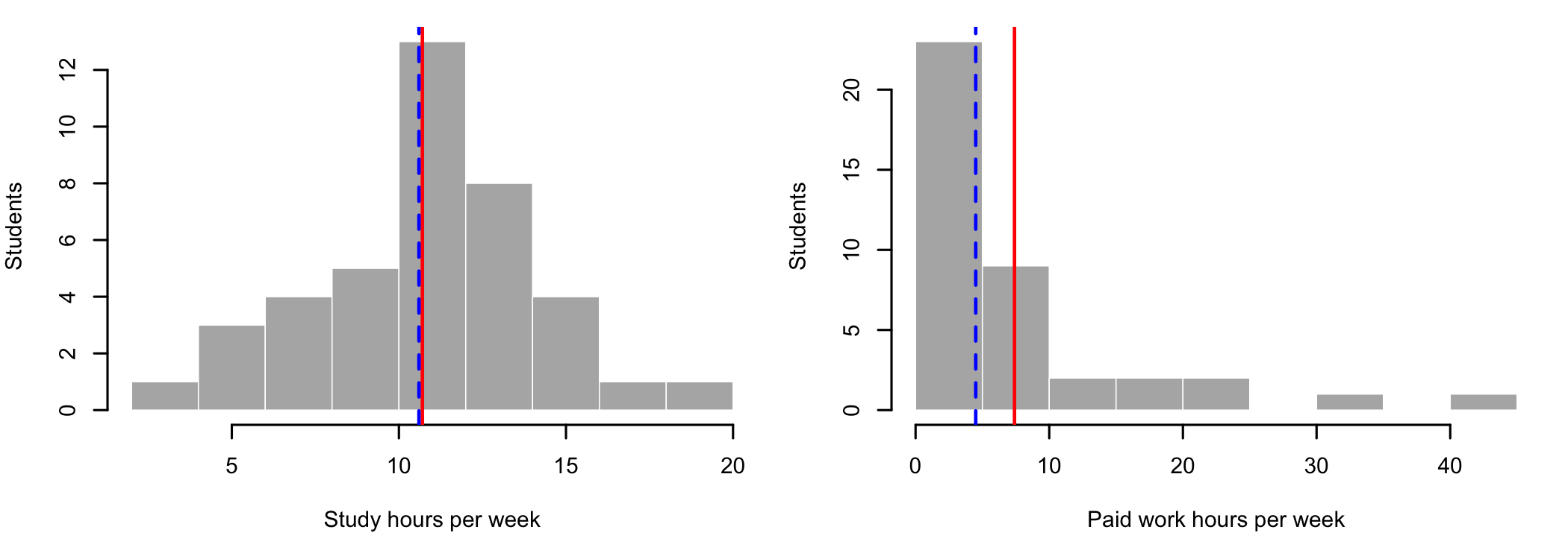
A histogram divides the range of the values into intervals of equal width, called bins, and draws a bar for each bin with a height equal to the number of values in it2121 The shape of a histogram depends on the number of bins. Too few bins hide the details of the distribution, and too many make it look ragged.. Figure 7.2 shows the two variables discussed above, with the mean in red and the median in blue (dashed). The study hours are spread approximately symmetrically around the center, and the mean and the median almost coincide. The hours of paid work are piled up at zero, with a long tail to the right, and the mean is pulled toward the tail.
21 The shape of a histogram depends on the number of bins. Too few bins hide the details of the distribution, and too many make it look ragged.
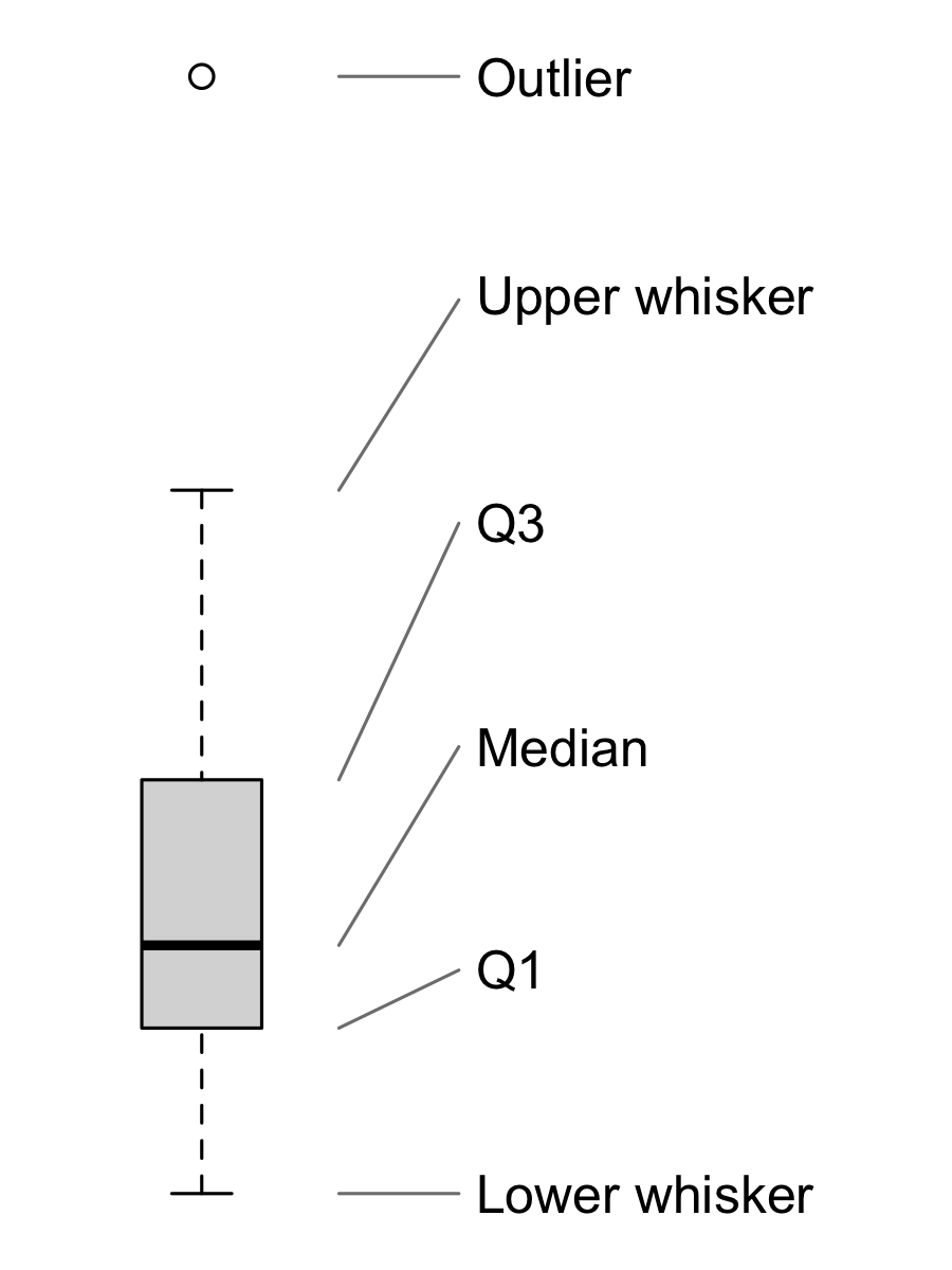
A box plot (Figure 7.3) shows the five-number summary of a numerical variable. The box spans the interquartile range, from Q_1 to Q_3, and the line inside it marks the median. The whiskers extend to the smallest and the largest values that are within 1.5 IQR of the box. Values beyond the whiskers are drawn as separate points and flagged as possible outliers2222 See Assumptions and Outliers for how outliers can be detected and handled..
22 See Assumptions and Outliers for how outliers can be detected and handled.
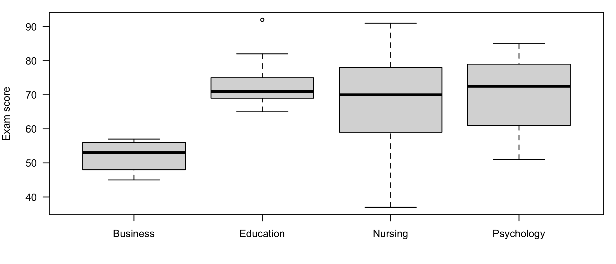
Box plots are especially useful for comparing groups. Figure 7.4 shows the exam scores of the students in each program.
7.6 Describing Groups
Most studies compare groups, and the descriptive statistics are then computed separately for each group. Table 7.4 summarizes the exam scores by program.
| Program | n | M | SD | Mdn | Range |
|---|---|---|---|---|---|
| Business | 4 | 52.00 | 5.29 | 53.00 | 45 - 57 |
| Education | 9 | 73.89 | 8.43 | 71.00 | 65 - 92 |
| Nursing | 13 | 67.23 | 17.02 | 70.00 | 37 - 91 |
| Psychology | 14 | 69.86 | 10.86 | 72.50 | 51 - 85 |
The Education students obtained the highest mean score (M = 73.89) and the Business students the lowest (M = 52.00). The differences between the groups describe only this sample. Whether they reflect real differences between the programs, or are only the result of which students happened to enroll in the course, is a question for an inferential test2323 With groups this small, and as unequal in size, any such test would have very little power. See Effect Size and Power., such as the one-way ANOVA.
23 With groups this small, and as unequal in size, any such test would have very little power. See Effect Size and Power.
7.7 Reporting the Results
When the study has several numerical variables, their descriptive statistics are usually reported in a table (Table 7.5). Report all the statistics with the same number of decimals2424 Two decimals are common. Counts and values measured in whole numbers, such as the minimum and maximum exam scores, need none..
24 Two decimals are common. Counts and values measured in whole numbers, such as the minimum and maximum exam scores, need none.
| Variable | M | SD | Mdn | Range |
|---|---|---|---|---|
| Paid work (hours per week) | 7.40 | 9.79 | 4.50 | 0 - 43 |
| Study (hours per week) | 10.70 | 3.37 | 10.60 | 3.3 - 19 |
| Exam score | 68.12 | 13.45 | 70.00 | 37 - 92 |
Finally, here is an example of how to write up the description of the sample in a publication. Statistical symbols, such as M, SD, and Mdn, are set in italics.
The participants were 40 students enrolled in a three-credit course, from Psychology (n = 14, 35%), Nursing (n = 13, 32%), Education (n = 9, 22%), and Business (n = 4, 10%). Most of them were in their sophomore year (n = 23, 58%). The students studied for the course on average 10.70 hours per week (SD = 3.37). The hours of paid work were positively skewed, Mdn = 4.50, IQR = 9.00, with 13 students (32%) not working at all. The mean score on the final exam was 68.12 (SD = 13.45). The students expected the course to be useful for their future work (Mdn = 3 on a scale from 1 to 5).
7.8 Summary
Descriptive statistics answer three questions about each variable: how often each value occurs, what a typical value is, and how spread out the values are. The scale of measurement decides which statistics can be used. Categorical variables are described by frequencies and percentages, and by the mode or, for ordinal data, the median. Numerical variables are described by the mean and the standard deviation when their distribution is approximately symmetric, and by the median and the interquartile range when it is skewed or has extreme values.
Of note is the fact that describing the data is not only a preliminary step. The frequencies show whether the groups are large enough to be compared, the comparison of the mean and the median signals skewed distributions, and the graphs reveal unusual values before they can distort the results of a test. All of these are checked again, more formally, in the next chapter, Assumptions and Outliers.