16 Repeated-Measures ANOVA
At a glance
- Question
- Do the means of three or more measurements of the same participants differ?
- Design
- One group measured three or more times, or under three or more conditions
- Dependent variable
- Interval or ratio
- Independent variable
- The measurements or conditions (a within-subjects factor)
- Assumptions
-
- The participants are independent of each other
- DV normally distributed at each measurement
- Sphericity: equal variances of the differences between all pairs of measurements (Mauchly’s test)
- Null hypothesis
- All population means are equal
- Test statistic
- F, with the participants’ differences removed from the error
- Effect size
- Partial \eta^{2}: .01 small, .06 medium, .14 large
- If conditions fail
-
- Sphericity is violated → The Greenhouse-Geisser or Huynh-Feldt correction of the degrees of freedom
- The DV is ordinal, or clearly not normal → Friedman test
- The DV has two categories, such as Yes and No → Cochran’s Q test
- Participants have missing measurements, or change at different rates → Multilevel model
- Include in the write-up
-
- The mean and standard deviation at each measurement
- The normality checks, and Mauchly’s test with the correction used
- F(df1, df2) = …, p = …, and \eta^{2}_{p}
- The trend contrasts or pairwise comparisons
Used to compare the means of a dependent (criterion) variable measured on the same participants three or more times, or under three or more conditions. The independent (predictor) variable is a within-subjects factor: each of its levels is a measurement of every participant11 See Between-Subjects vs. Within-Subjects Designs.. It extends the paired samples t-Test the same way the one-way ANOVA extends the independent samples t-Test.
Repeated measures appear in two kinds of designs:
- Measurements over time, such as the anxiety of patients before, during, and after a treatment, or the reading skills of children at the beginning, middle, and end of a school year;
- Measurements under several conditions, such as the reaction times of the same participants to three kinds of stimuli, presented one after the other.
Because each participant is compared with themselves, the differences between the participants, such as their abilities or their personalities, are removed from the comparison. The repeated-measures design is therefore usually more powerful than a between-subjects design with the same number of participants, and needs fewer participants to reach the same power22 The gain depends on how strongly the measurements of the same participant are related. When they are only weakly related, the advantage is small.. The price is that measuring the same participants several times can introduce carryover effects33 Practice, fatigue, boredom, or the participants guessing the purpose of the study.. When the conditions can be presented in any order, these effects are controlled by counterbalancing, presenting the conditions in different orders to different participants. Measurements over time cannot be counterbalanced, and their changes may be due to the passing of time as much as to the treatment44 A control group, measured at the same times without the treatment, solves the problem. The resulting design, with one between-subjects and one within-subjects factor, is called a mixed design..
2 The gain depends on how strongly the measurements of the same participant are related. When they are only weakly related, the advantage is small.
3 Practice, fatigue, boredom, or the participants guessing the purpose of the study.
4 A control group, measured at the same times without the treatment, solves the problem. The resulting design, with one between-subjects and one within-subjects factor, is called a mixed design.
The repeated-measures ANOVA has two alternatives for data that do not meet its assumptions, and a more flexible approach for measurements over time. Table 16.1 shows which test to use.
| Data | Test |
|---|---|
| Normal data, three or more measurements | Repeated-measures ANOVA |
| Ordinal or clearly not normal data | Friedman test |
| Two values only, such as Yes and No | Cochran’s Q test |
| Measurements over time, with individual change or missing measurements | Multilevel model |
| Two measurements only | Paired samples t-Test, Wilcoxon signed-rank test, or McNemar’s test |
| A between-subjects factor as well | Mixed designs |
16.1 The Theory
16.1.1 Partitioning the Variance
In a between-subjects design, the differences between the participants are part of the error. In a repeated-measures design they can be measured, because each participant contributes several scores, and removed from the error. The total sum of squares is first divided into the variability between the participants and the variability within the participants:
SS_{T} = SS_{B} + SS_{W}
SS_{B}, computed from the differences between the participants’ mean scores, represents the individual differences. It is not of interest and is set aside. SS_{W}, the variability of each participant’s scores around their own mean, is then divided into the part explained by the conditions, SS_{M}, and the part left unexplained, SS_{R}:
SS_{W} = SS_{M} + SS_{R}
With k measurements of n participants, the conditions are tested with:
F = \frac{MS_{M}}{MS_{R}} = \frac{SS_{M} / (k - 1)}{SS_{R} / [(k - 1)(n - 1)]}
Of note is the fact that SS_{M} is computed exactly as in the one-way ANOVA, from the differences between the condition means. The gain in power comes entirely from the error term, which no longer includes the individual differences.
16.1.2 Sphericity
The repeated-measures ANOVA replaces the assumption of homogeneity of variances with sphericity: the variances of the differences between all pairs of conditions must be equal55 With four measurements there are six such differences (week 1 minus week 2, week 1 minus week 3, and so on). With only two measurements there is only one difference, and the assumption is always met..
5 With four measurements there are six such differences (week 1 minus week 2, week 1 minus week 3, and so on). With only two measurements there is only one difference, and the assumption is always met.
Sphericity is often violated in measurements over time, because measurements close in time tend to be more similar than measurements far apart. When it is violated, the F test becomes too liberal: it rejects H0 more often than \alpha. Sphericity is tested with Mauchly’s test. When the test is significant, the degrees of freedom of the F test are multiplied by a correction factor, epsilon (\varepsilon), which is 1 when sphericity holds and smaller the more it is violated. Two estimates of \varepsilon are common:
- Greenhouse-Geisser, which tends to over-correct, especially when \varepsilon is close to 1;
- Huynh-Feldt, which tends to under-correct.
A common rule is to use the Greenhouse-Geisser correction when its \varepsilon is below .75, and the Huynh-Feldt correction otherwise.
16.1.3 Effect Size
The effect size is the partial eta squared, the variability explained by the conditions relative to that variability plus the error:
\eta^{2}_{p} = \frac{SS_{M}}{SS_{M} + SS_{R}}
Because the individual differences are not part of the denominator, \eta^{2}_{p} is usually larger in a repeated-measures design than in a between-subjects design with the same data. It is read with the usual guidelines: .01 small, .06 medium, and .14 or more large66 The generalized eta squared (\eta^{2}_{G}) is sometimes reported instead, because it can be compared across within- and between-subjects designs..
6 The generalized eta squared (\eta^{2}_{G}) is sometimes reported instead, because it can be compared across within- and between-subjects designs.
16.2 Assumptions
- Independence of the participants
- Ensured by the design of the study. The scores of the same participant are related, by design, but the participants must be independent of each other;
- Violated when the participants influence each other.
- Normality
- Detected using q-q plots and tests of normality of the scores at each measurement;
- Violated when the distributions are strongly skewed or have outliers.
- Sphericity
- Detected using Mauchly’s test;
- Violated when the variances of the differences between the conditions are not equal. The degrees of freedom are then corrected.
The Friedman test is the rank-based alternative to the repeated-measures ANOVA, used when the dependent variable is ordinal or not normally distributed. A multilevel model is an alternative that does not require sphericity and can use participants with missing measurements. Both are presented at the end of the chapter.
16.3 The Study
A university counseling center offered an eight-week mindfulness program to graduate students. Twenty-four students who joined the program completed a perceived stress questionnaire (scored from 0 to 40, higher scores meaning more stress) at the start of the program (week 0), in the middle of it (week 4), at the end of it (week 8), and a month after it ended (week 12). The question asked is: Did the students’ stress change over the course of the program, and did the change last after the program ended? The data set77 Column labels are: student, week0, week4, week8, and week12. was made up for this example. The first few rows of the data set are shown in Table 16.288 The data is stored in the wide format, with one row for each student and one column for each measurement. This is the natural way to enter repeated measures, and the format used by some of the analyses below. Other analyses, and most graphs, need the long format, with one row for each measurement and a column that identifies the student..
7 Column labels are: student, week0, week4, week8, and week12.
8 The data is stored in the wide format, with one row for each student and one column for each measurement. This is the natural way to enter repeated measures, and the format used by some of the analyses below. Other analyses, and most graphs, need the long format, with one row for each measurement and a column that identifies the student.
| Student | Week 0 | Week 4 | Week 8 | Week 12 |
|---|---|---|---|---|
| 1 | 19 | 11 | 10 | 13 |
| 2 | 31 | 23 | 19 | 24 |
| 3 | 24 | 18 | 10 | 11 |
| 4 | 30 | 23 | 25 | 19 |
| 5 | 27 | 19 | 10 | 9 |
| 6 | 25 | 23 | 23 | 20 |
     student week stress
1.0        1    0     19
1.4        1    4     11
1.8        1    8     10
1.12       1   12     13
2.0        2    0     31
2.4        2    4     23
Hypotheses.
- Null hypothesis (H0): In the population, the mean stress score is the same at the four measurements (\mu_{0} = \mu_{4} = \mu_{8} = \mu_{12}).
- Alternative hypothesis (H1): The mean stress score differs between at least two of the measurements.
Decision criteria. The significance level is set at \alpha = .05. With k = 4 measurements of n = 24 students, the test has 3 and 3 \times 23 = 69 degrees of freedom, corrected if sphericity is violated. H0 is rejected if the p-value is smaller than \alpha. The effect size is \eta^{2}_{p}.
16.3.1 Describing the Measurements
| Measurement | M | SD |
|---|---|---|
| Week 0 | 26.92 | 5.59 |
| Week 4 | 22.71 | 5.53 |
| Week 8 | 20.58 | 6.38 |
| Week 12 | 20.54 | 7.44 |
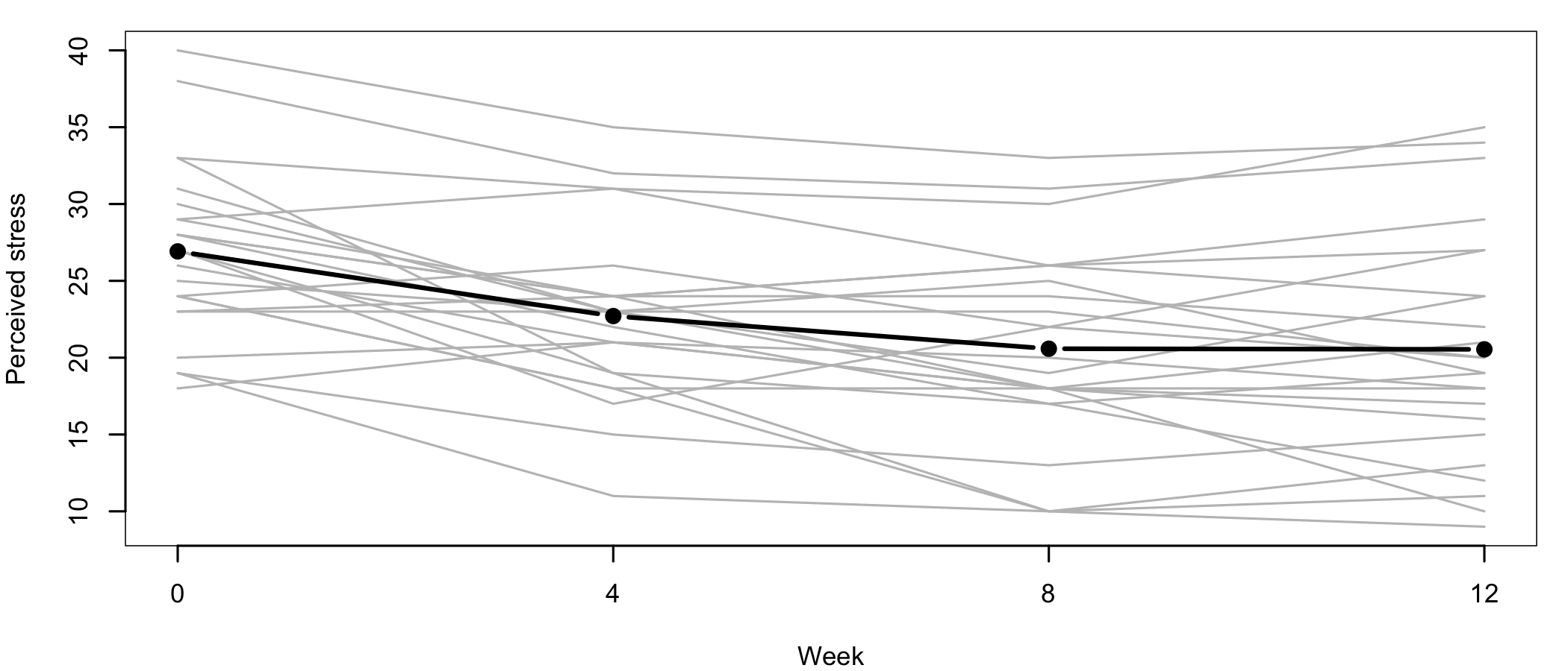
The mean stress score dropped from 26.92 at the start of the program to 20.58 at its end, and stayed at about the same level a month later (Table 16.3). Figure 16.1 shows the scores of each student, which tell more than the means alone. The students started from very different levels of stress, but most of them followed the same downward path. Of note is the fact that the lines spread out over time: the program helped some students much more than others. This is a first sign that sphericity may not hold.
16.3.2 Checking the Assumptions
The independence of the participants is supported by the design: each student filled in the questionnaire on their own.
    week0     week4     week8    week12
0.4634599 0.3454672 0.4028126 0.4127644
The stress scores do not depart significantly from normality at any measurement (Shapiro-Wilk p-values between .345 and .463). Sphericity is tested together with the ANOVA.
16.3.3 The Repeated-Measures ANOVA
Univariate Type III Repeated-Measures ANOVA Assuming Sphericity

            Sum Sq num Df Error SS den Df F value    Pr(>F)
(Intercept)  49413      1  2944.12     23 386.026 7.123e-16 ***
week           646      3   688.46     69  21.583 5.730e-10 ***
---
Signif. codes:  0 '***' 0.001 '**' 0.01 '*' 0.05 '.' 0.1 ' ' 1


Mauchly Tests for Sphericity

     Test statistic  p-value
week        0.53073 0.017314


Greenhouse-Geisser and Huynh-Feldt Corrections
 for Departure from Sphericity

      GG eps Pr(>F[GG])
week 0.69079  1.576e-07 ***
---
Signif. codes:  0 '***' 0.001 '**' 0.01 '*' 0.05 '.' 0.1 ' ' 1

        HF eps   Pr(>F[HF])
week 0.7603494 4.437939e-08
The output has three parts:
- The univariate test, assuming sphericity. The week row shows F(3, 69) = 21.5899 The (Intercept) row tests whether the overall mean is zero, and its Error SS, 2944.1, is the variability between the students, SS_{B}, which was removed from the error term.;
9 The (Intercept) row tests whether the overall mean is zero, and its Error SS, 2944.1, is the variability between the students, SS_{B}, which was removed from the error term.
- Mauchly’s test. It is significant (p = .017): the assumption of sphericity is violated;
- The corrections. The Greenhouse-Geisser \varepsilon is 0.69 and the Huynh-Feldt \varepsilon is 0.76.
Because \varepsilon is below .75, the Greenhouse-Geisser correction is used. Both degrees of freedom are multiplied by \varepsilon: 3 \times 0.69 = 2.07 and 69 \times 0.69 = 47.66. The value of F does not change, but its p-value is computed with the corrected degrees of freedom.
Decision. With F(2.07, 47.66) = 21.58, p < .001, Greenhouse-Geisser corrected, the p-value is smaller than \alpha = .05. The null hypothesis is rejected and the alternative hypothesis accepted: the mean stress scores differ between the measurements.
Effect size. \eta^{2}_{p} = 0.48, a large effect. The weeks explain 48% of the variability within the students that is not due to error.
16.3.4 Following Up
As in the one-way ANOVA, a significant F is followed up with planned contrasts or with post hoc tests.
Trend analysis. When the levels of the factor are points in time, the most natural planned contrasts are polynomial contrasts, which test the shape of the change. With four equally spaced measurements, the linear contrast (weights -3, -1, 1, 3) tests a steady increase or decrease, and the quadratic contrast (weights 1, -1, -1, 1) tests a curve, a change that speeds up or slows down. In a repeated-measures design, a contrast is computed for each participant, as the weighted sum of their scores, and tested against zero with a one-sample t-Test.
    One Sample t-test

data:  my.lin
t = -5.3415, df = 23, p-value = 2.008e-05
alternative hypothesis: true mean is not equal to 0
95 percent confidence interval:
 -29.47977 -13.02023
sample estimates:
mean of x
   -21.25
    One Sample t-test

data:  my.quad
t = 4.1027, df = 23, p-value = 0.0004357
alternative hypothesis: true mean is not equal to 0
95 percent confidence interval:
 2.065781 6.267552
sample estimates:
mean of x
 4.166667
Both contrasts are significant. The linear contrast, t(23) = -5.34, p < .001, shows that stress decreased over the weeks. The quadratic contrast, t(23) = 4.10, p < .001, shows that the decrease was not steady: it was steep at the beginning and leveled off toward the end, as Figure 16.1 suggests.
Pairwise comparisons. All pairs of measurements are compared with paired t-Tests, with a Bonferroni correction for the six comparisons:
    Pairwise comparisons using paired t tests

data:  st.long$stress and st.long$week

   0       4       8
4  0.00035 -       -
8  1.1e-05 0.02666 -
12 0.00019 0.13192 1.00000

P value adjustment method: bonferroni
Stress at the start of the program was higher than at all later measurements (all p-values < .001). Stress also decreased from the middle to the end of the program (p = .027). The scores at the end of the program and a month later did not differ significantly (p = 1.000): the data show no sign that stress went back up after the program ended1010 This is not proof that the reduction lasted, since a small increase could have gone undetected. Showing that the scores stayed the same takes an equivalence test, with a margin set in advance..
10 This is not proof that the reduction lasted, since a small increase could have gone undetected. Showing that the scores stayed the same takes an equivalence test, with a margin set in advance.
16.3.5 Reporting the Results
A one-way repeated-measures ANOVA compared the perceived stress of 24 graduate students at the start (week 0), middle (week 4), and end (week 8) of an eight-week mindfulness program, and a month after it ended (week 12). The scores did not depart significantly from normality at any measurement (Shapiro-Wilk p-values between .345 and .463). Mauchly’s test indicated that the assumption of sphericity was violated, W = .53, p = .017, and the degrees of freedom were corrected with the Greenhouse-Geisser estimate (ε = .69). Stress changed significantly over time, F(2.07, 47.66) = 21.58, p < .001, η2p = .48. Stress decreased from week 0 (M = 26.92, SD = 5.59) to week 8 (M = 20.58, SD = 6.38), with significant linear and quadratic trends, and Bonferroni-corrected comparisons showed no significant change between week 8 and week 12 (M = 20.54, SD = 7.44, p = 1.000).
16.4 The Friedman Test
At a glance
- Use instead of
- The repeated-measures ANOVA, when the DV is ordinal or clearly not normal
- Question
- Do the scores tend to change across three or more measurements of the same participants?
- Design
- One group measured three or more times, or under three or more conditions
- Dependent variable
- Ordinal, interval, or ratio
- Assumptions
-
- The participants are independent of each other
- Null hypothesis
- The ranks of the measurements are the same in the population
- Test statistic
- \chi^{2}, with k - 1 degrees of freedom
- Effect size
- Kendall’s W, from 0 (no agreement in how participants rank the measurements) to 1
- Include in the write-up
-
- The median at each measurement
- Why the rank-based test was used
- \chi^{2}(df) = …, p = …, and Kendall’s W
- The pairwise Wilcoxon signed-rank tests, with a Bonferroni correction
The Friedman test is the rank-based alternative to the repeated-measures ANOVA. The scores of each participant are ranked from the lowest to the highest, and the test compares the mean ranks of the conditions. It does not assume normality or sphericity, and can be used with ordinal data.
    Friedman rank sum test

data:  as.matrix(st[, -1])
Friedman chi-squared = 27.258, df = 3, p-value = 5.199e-06
The Friedman test leads to the same conclusion as the ANOVA, \chi^{2}(3) = 27.26, p < .001. Its effect size is Kendall’s W, W = \chi^{2} / [n(k - 1)] = 0.381111 W ranges from 0 (no agreement among the participants in how they rank the conditions) to 1 (complete agreement).. A significant result is followed up with pairwise Wilcoxon signed-rank tests, with a Bonferroni correction.
11 W ranges from 0 (no agreement among the participants in how they rank the conditions) to 1 (complete agreement).
16.5 Cochran’s Q Test
At a glance
- Use instead of
- The repeated-measures ANOVA or the Friedman test, when the variable has only two values
- Question
- Does the proportion of Yes answers change across three or more measurements?
- Design
- One group classified three or more times
- Variable
- Nominal, two categories
- Assumptions
-
- The participants are independent of each other
- Null hypothesis
- The proportion of Yes answers is the same at all measurements
- Test statistic
- Q, compared with a chi-square distribution with k - 1 degrees of freedom
- Effect size
- \eta^{2}_{Q} = Q / [n(k - 1)], from 0 to 1
- Include in the write-up
-
- The number of participants, and the proportion of Yes at each measurement
- Q(df) = …, p = …, and \eta^{2}_{Q}
- The pairwise McNemar’s tests, with a Bonferroni correction
When the variable measured three or more times has only two values, such as Yes and No, neither the ANOVA nor the Friedman test can be used. Cochran’s Q test compares the proportion of Yes answers across the measurements. It extends McNemar’s test to three or more measurements, the same way the repeated-measures ANOVA extends the paired samples t-Test.
An example: at weeks 4, 8, and 12, the same 24 students were also asked whether they had practiced mindfulness on at least three days in the past week. The question asked is: Did the proportion of students who practiced regularly change over time, in particular after the program ended? The data set1212 Column labels are: student, week4, week8, and week12. was made up for this example.
12 Column labels are: student, week4, week8, and week12.
 week4  week8 week12
    19     19      6
Hypotheses.
- Null hypothesis (H0): In the population, the proportion of students who practice regularly is the same at all three measurements.
- Alternative hypothesis (H1): In the population, the proportion of students who practice regularly differs between at least two of the measurements.
Decision criteria. The significance level is set at \alpha = .05. Like McNemar’s test, Cochran’s Q uses only the students whose answers changed: a student who answered Yes every time, or No every time, carries no information about change. The statistic is computed from the number of Yes answers at each measurement, C_{j}, and for each student, R_{i}:
Q = \frac{(k - 1)\left[k\sum C_{j}^{2} - N^{2}\right]}{kN - \sum R_{i}^{2}}
where k is the number of measurements and N the total number of Yes answers. Q follows a chi-square distribution with k - 1 degrees of freedom. H0 is rejected if the p-value is smaller than \alpha. The effect size is \eta^{2}_{Q} = Q / [n(k - 1)], which, like Kendall’s W, ranges from 0 to 1.
           Q           df            p
1.609524e+01 2.000000e+00 3.198626e-04
3 of the 24 students gave the same answer all three times and do not contribute to the test.
Decision. With Q(2) = 16.10, p < .001, H0 is rejected: the proportion of students who practiced regularly changed over time.
Effect size. \eta^{2}_{Q} = 0.34. 79% of the students practiced regularly at week 4 and 79% at week 8, but only 25% a month after the program ended.
A significant result is followed up with pairwise McNemar’s tests, with a Bonferroni correction.
 week4 vs. week8 week4 vs. week12 week8 vs. week12
           1.000            0.011            0.011
The proportions at weeks 4 and 8 do not differ significantly (p > .999), and both are higher than at week 12 (p = .011 and p = .011). Most students kept practicing during the program, but many stopped once it ended, even though their stress stayed low a month later.
Cochran’s Q test compared the proportion of 24 graduate students who practiced mindfulness on at least three days a week at the middle (week 4) and the end (week 8) of an eight-week program, and a month after it ended (week 12). The proportion changed significantly over time, Q(2) = 16.10, p < .001, η2Q = .34. Bonferroni-corrected McNemar’s tests showed that fewer students practiced regularly at week 12 (25%) than at week 4 (79%) and week 8 (79%), which did not differ significantly.
16.6 The Multilevel Approach
At a glance
- Question
- How do the scores change over time, and does the change differ between participants?
- Design
- Participants measured repeatedly, possibly at different times or with missing measurements
- Criterion
- Interval or ratio
- Predictors
- Time, and any characteristics of the participants
- Assumptions
-
- Normally distributed residuals and random effects
- The model includes the random effects the data needs (intercepts, and slopes if the change varies)
- Null hypothesis
- For each fixed effect, a coefficient of zero; for a random effect, no variation between participants
- Test statistic
- t for the fixed effects; a likelihood ratio \chi^{2} to compare models
- Effect size
- The fixed effects in the units of the criterion, and the standard deviations of the random effects
- Include in the write-up
-
- The random effects in the model, and why
- The fixed effects with their tests
- The model comparison, \\chi^{2}(df) = …, p = …
Repeated measures can also be seen as nested data: the measurements are nested within the participants. Multilevel models1313 Also called mixed-effects models or hierarchical linear models. analyze such data with a regression in which each participant has their own intercept, called a random intercept. The random intercepts capture the individual differences that the repeated-measures ANOVA removes as SS_{B}.
13 Also called mixed-effects models or hierarchical linear models.
Multilevel models have several advantages over the repeated-measures ANOVA:
- They do not require sphericity, and can model how the measurements are related to each other;
- They can use participants with missing measurements, while the ANOVA drops every participant with at least one missing score1414 This works when whether a score is missing can be explained by the data that was observed, such as the earlier scores of the same participant (missing at random). When students drop out because their stress went up, and this is not visible in their earlier scores, no model can fully correct for it.;
14 This works when whether a score is missing can be explained by the data that was observed, such as the earlier scores of the same participant (missing at random). When students drop out because their stress went up, and this is not visible in their earlier scores, no model can fully correct for it.
- They can let the effect of time vary from one participant to another, with random slopes;
- The measurements do not need to be at the same times for all participants.
In exchange, they have assumptions of their own:
- Normally distributed residuals
- Detected using a q-q plot or a test of normality of the residuals of the model;
- Violated when the distribution is strongly skewed or has outliers.
- Normally distributed random effects, such as the participants’ intercepts and slopes
- Detected using a q-q plot or a test of normality of the estimated random effects;
- Violated when a few participants are very different from the others.
- The random effects the data needs are in the model
- Detected by comparing models with and without them, as shown below for the random slopes;
- Violated when, for example, the change over time varies between the participants but the model gives them all the same slope.
The model is built step by step. A baseline model, with only the random intercepts, is compared with a model that adds the weeks. The comparison uses a likelihood ratio test, and the model with the smaller AIC fits the data better1515 The models are fitted by full maximum likelihood, which is required when models with different fixed effects are compared..
15 The models are fitted by full maximum likelihood, which is required when models with different fixed effects are compared.
      Model df      AIC      BIC    logLik   Test  L.Ratio p-value
my.m0     1  3 604.0790 611.7721 -299.0395
my.m1     2  6 562.4253 577.8114 -275.2126 1 vs 2 47.65372  <.0001
Adding the weeks improves the model significantly, \chi^{2}(3) = 47.65, p < .001, and lowers the AIC from 604.1 to 562.4. The coefficients of the model compare each week with week 0:
                Value Std.Error DF   t-value      p-value
(Intercept) 26.916667 1.2826503 69 20.985195 1.145488e-31
week4       -4.208333 0.9118505 69 -4.615157 1.760876e-05
week8       -6.333333 0.9118505 69 -6.945583 1.668977e-09
week12      -6.375000 0.9118505 69 -6.991277 1.379484e-09
On average, stress decreased by 4.21 points from week 0 to week 4, by 6.33 points to week 8, and by 6.37 points to week 12, all significant.
The plot of the students’ scores (Figure 16.1) showed that the program helped some students more than others. A model with random slopes lets the rate of change over time differ from one student to another1616 Here, the weeks are entered as a number, so that each student has their own slope of stress over time..
16 Here, the weeks are entered as a number, so that each student has their own slope of stress over time.
      Model df      AIC      BIC    logLik   Test  L.Ratio p-value
my.m1     1  6 562.4253 577.8114 -275.2126
my.m2     2  8 548.5571 569.0719 -266.2785 1 vs 2 17.86823   1e-04
The model with random slopes fits the data significantly better1717 The usual chi-square test is conservative here: under the null hypothesis the variance of the slopes is zero, at the edge of its possible values, and the p-value comes out too large. A significant result, as here, is therefore safe., \chi^{2}(2) = 17.87, p < .001. The standard deviation of the slopes, 0.40 points per week, means that over twelve weeks the change in stress of a typical student could differ from the average change by about 4.8 points. This variation between the students is what violated the sphericity assumption of the ANOVA. The multilevel model does not need to correct for it, because it describes it.
17 The usual chi-square test is conservative here: under the null hypothesis the variance of the slopes is zero, at the edge of its possible values, and the p-value comes out too large. A significant result, as here, is therefore safe.
No assumption of the final model is clearly violated: neither its residuals (Shapiro-Wilk p = .812) nor the students’ random intercepts (p = .461) and slopes (p = .569) depart significantly from normality.
16.7 Summary
The repeated-measures ANOVA compares three or more measurements of the same participants. By removing the differences between the participants from the error, it is more powerful than a between-subjects design. In exchange, it requires sphericity, which is often violated in measurements over time and is then corrected with the Greenhouse-Geisser or Huynh-Feldt estimates of \varepsilon. In the mindfulness study, the students’ stress decreased during the program, most of it in the first weeks, and the decrease lasted a month after the program ended. The rank-based Friedman test replaces the ANOVA for ordinal or clearly non-normal data, and Cochran’s Q test for a variable with only two values, such as whether the students kept practicing.
Of note is the fact that the study had no control group. The students’ stress may have decreased for reasons other than the program, such as the end of a busy part of the semester. The design shows that stress changed, not that the program changed it. Adding a control group, measured at the same times, would turn the study into a mixed design, with one between-subjects and one within-subjects factor.