12 ANOVA: Analysis of Variance
At a glance
- Question
- Do the means of two or more independent groups differ?
- Design
- Two or more independent groups, one measurement of each participant
- Dependent variable
- Interval or ratio
- Independent variable
- Nominal, two or more levels
- Assumptions
-
- Independent observations: each participant belongs to one group only
- DV normally distributed in each group
- Equal variances in the groups (Levene’s test)
- Null hypothesis
- All population means are equal
- Test statistic
- F, with k - 1 and N - k degrees of freedom
- Effect size
- \eta^{2} or \omega^{2}: .01 small, .06 medium, .14 large
- If conditions fail
-
- The variances are not equal → Welch’s ANOVA
- The DV is ordinal, or clearly not normal in a small sample → Kruskal-Wallis test
- Include in the write-up
-
- The size, mean, and standard deviation of each group
- The assumption checks: normality in each group (Shapiro-Wilk p = …) and Levene’s test
- F(df1, df2) = …, p = …, and \omega^{2}
- The planned contrasts or post hoc tests that follow a significant F
Used to compare the means of a dependent (criterion) variable between two or more groups defined by an independent (predictor) variable measured on a nominal scale. The test computes an F value, the ratio between the variation between the groups and the variation within the groups, to determine if the observed differences between the group means represent differences between the populations the samples were drawn from (alternative hypothesis, H1), or if they are due purely to chance (null hypothesis, H0).
With only two groups, the one-way ANOVA and the independent samples t-Test lead to the same conclusion11 With two groups, F = t^2 and the two tests have the same p-value. This holds for the t-Test that assumes equal variances (Student’s), not for Welch’s version.. The ANOVA becomes necessary when the independent variable has three or more levels. This chapter covers the one-way ANOVA, with a single independent variable. Designs with two or more independent variables are discussed in the chapter on Factorial ANOVA.
1 With two groups, F = t^2 and the two tests have the same p-value. This holds for the t-Test that assumes equal variances (Student’s), not for Welch’s version.
The one-way ANOVA has two alternatives for data that do not meet its assumptions, and related designs have chapters of their own. Table 12.1 shows which test to use.
| Data or design | Test |
|---|---|
| One independent variable, normal data, equal variances | One-way ANOVA |
| One independent variable, normal data, unequal variances | Welch’s ANOVA |
| One independent variable, ordinal or clearly not normal data | Kruskal-Wallis test |
| Two or more independent variables | Factorial ANOVA |
| A covariate whose effect is removed | ANCOVA |
| Two or more dependent variables | MANOVA |
| The same participants measured three or more times | Repeated-measures ANOVA |
12.1 Why Not Several t-Tests?
With three groups, we could compare them two at a time with three t-Tests. With four groups, six t-Tests would be needed. In general, k groups can be paired in c = k(k - 1)/2 different ways. The problem is that each test carries its own risk of a Type I error22 Rejecting a null hypothesis that is true. See Hypothesis Testing.. When each test is run at \alpha = .05, the probability of making at least one Type I error in the whole set of tests, called the familywise error rate, is, if the tests are independent:
2 Rejecting a null hypothesis that is true. See Hypothesis Testing.
\alpha_{FW} = 1 - (1 - \alpha)^c
| Groups | t-Tests | Familywise error rate |
|---|---|---|
| 2 | 1 | 0.050 |
| 3 | 3 | 0.143 |
| 4 | 6 | 0.265 |
| 5 | 10 | 0.401 |
| 6 | 15 | 0.537 |
Table 12.2 shows how quickly the risk grows. With four groups, the chances of declaring at least one difference that does not exist are already 26%, not 5%. The ANOVA avoids the problem by testing all the groups at once, with a single test, called an omnibus test. Of note is the fact that the omnibus test only tells us whether the group means differ. Finding out which groups differ requires the follow-up procedures discussed later in this chapter, which keep the familywise error rate under control.
12.2 The Theory
12.2.1 Partitioning the Variance
As in Simple Linear Regression, the analysis starts from the total variability in the data, the squared deviations of all scores from the grand mean \bar{Y}33 The mean of all scores, regardless of group.. This variability is split into two parts:
3 The mean of all scores, regardless of group.
- Model (between-groups) sum of squares (SS_{M}), the part explained by the groups. It compares each group mean \bar{Y}_k with the grand mean, weighted by the size of the group n_k: SS_{M} = \sum n_k(\bar{Y}_k - \bar{Y})^2;
- Residual (within-groups) sum of squares (SS_{R}), the part the groups cannot explain. It compares each score with the mean of its own group: SS_{R} = \sum(Y_{ik} - \bar{Y}_k)^2.
Together they add up to the total sum of squares:
SS_{T} = SS_{M} + SS_{R}
If the groups do not differ in the population, the group means will be close to each other and to the grand mean, and SS_{M} will be small compared with SS_{R}. If they do differ, the group means will be spread out and SS_{M} will be large.
12.2.2 The F Ratio
The two sums of squares cannot be compared directly, because they are computed from different numbers of values. Each is first divided by its degrees of freedom, resulting in the mean squares (MS). With k groups and N participants in total:
MS_{M} = \frac{SS_{M}}{k - 1} \qquad MS_{R} = \frac{SS_{R}}{N - k} \qquad F = \frac{MS_{M}}{MS_{R}}
MS_{R} estimates the variance of the scores inside the groups, the “noise” in the data. MS_{M} estimates the same noise plus any real differences between the groups. When H0 is true, the two estimate the same quantity and F is close to 1. The larger the value of F, the stronger the evidence that the groups differ.
12.2.3 ANOVA Is a Regression
The ANOVA and the regression are usually taught as separate techniques, but they are the same model, the general linear model. An independent variable with k groups can be entered in a regression as k - 1 dummy variables, coded 0 or 1. One group, the reference group, is coded 0 on all of them. With four groups:
\hat{Y}_i = b_0 + b_1 D_{1i} + b_2 D_{2i} + b_3 D_{3i}
The intercept b_0 is the mean of the reference group, and each slope is the difference between the mean of one of the other groups and the mean of the reference group. The F test of the regression model is the F test of the ANOVA, and the R^2 of the model is the effect size of the ANOVA. We will check this with the example below.
12.2.4 Effect Size
The effect size of the ANOVA is eta squared (\eta^{2}), the share of the total variance explained by the groups. It is the same quantity as the R^2 of a regression:
\eta^{2} = \frac{SS_{M}}{SS_{T}}
Values around .01 indicate a small effect, .06 a medium effect, and .14 or more a large effect. Like R^2, \eta^{2} describes the sample and tends to overestimate the effect in the population, especially in small samples. Omega squared (\omega^{2}) corrects this bias and is read with the same guidelines44 The correction is larger when the samples are small. With large samples, \eta^{2} and \omega^{2} are very close.:
4 The correction is larger when the samples are small. With large samples, \eta^{2} and \omega^{2} are very close.
\omega^{2} = \frac{SS_{M} - (k - 1)MS_{R}}{SS_{T} + MS_{R}}
12.3 Assumptions
- Independence of observations
- Usually ensured by the design of the study55 E.g., each participant belongs to only one group and is measured independently of the other participants.;
5 E.g., each participant belongs to only one group and is measured independently of the other participants.
- Violated when the participants influence each other or are measured more than once66 Repeated measurements of the same participants require a repeated-measures design and its own analysis, the Repeated-Measures ANOVA..
6 Repeated measurements of the same participants require a repeated-measures design and its own analysis, the Repeated-Measures ANOVA.
- Usually ensured by the design of the study55 E.g., each participant belongs to only one group and is measured independently of the other participants.;
- The dependent variable (DV) is normally distributed in each group
- Detected using histograms, q-q plots, and tests of normality for each group;
- Violated when the distributions are strongly skewed or have outliers. With groups of similar size the F test is fairly robust to moderate departures from normality.
- Homogeneity of variances
- Detected using Levene’s test77 See Homogeneity of Variances or Homoscedasticity. and by comparing the standard deviations of the groups;
- Violated when the variances differ, which is more serious when the groups also differ in size.
When the variances are not equal, Welch’s ANOVA can be used instead. When the dependent variable is not normally distributed, or is ordinal, the Kruskal-Wallis test, the rank-based alternative to the one-way ANOVA, can be used. Both are presented at the end of the chapter.
12.4 The Study
The instructor of a first-year writing course wanted to know which kind of feedback helps students most when they revise an essay. The 60 students enrolled in the course wrote a first draft and were then randomly assigned to one of four groups of 15 students. The first group received no feedback (None). The students in the second group exchanged drafts and commented on each other’s work (Peer). The third group received written comments from the instructor (Written), and the fourth discussed their draft with the instructor in a short one-on-one meeting (Conference). Two weeks later, all students submitted a revised essay, which was scored from 0 to 100 by a grader who did not know which group the students belonged to88 A blind grader cannot be influenced, even unintentionally, by knowing which students received which treatment.. The data set99 Column labels are: student, feedback, and score. was made up for this example. The first few rows of the data set are shown in Table 12.3.
8 A blind grader cannot be influenced, even unintentionally, by knowing which students received which treatment.
9 Column labels are: student, feedback, and score.
| Student | Feedback | Revision score |
|---|---|---|
| 1 | None | 58 |
| 2 | None | 80 |
| 3 | None | 55 |
| 4 | None | 47 |
| 5 | None | 52 |
| 6 | None | 55 |
Hypotheses.
- Null hypothesis (H0): In the population, the mean revision score is the same for all four kinds of feedback (\mu_{None} = \mu_{Peer} = \mu_{Written} = \mu_{Conference}).
- Alternative hypothesis (H1): At least one group mean differs from the others.
Decision criteria. The significance level is set at \alpha = .05. The F test has no direction: a larger F means larger differences between the groups relative to the variation within them, whatever their direction. With k = 4 groups and N = 60 students, the test has 3 and 56 degrees of freedom. H0 is rejected if the p-value is smaller than \alpha. The effect size is \eta^{2}, together with \omega^{2}.
12.4.1 Describing the Groups
| Feedback | n | M | SD |
|---|---|---|---|
| None | 15 | 60.60 | 9.43 |
| Peer | 15 | 67.13 | 8.11 |
| Written | 15 | 74.80 | 6.39 |
| Conference | 15 | 73.40 | 6.86 |
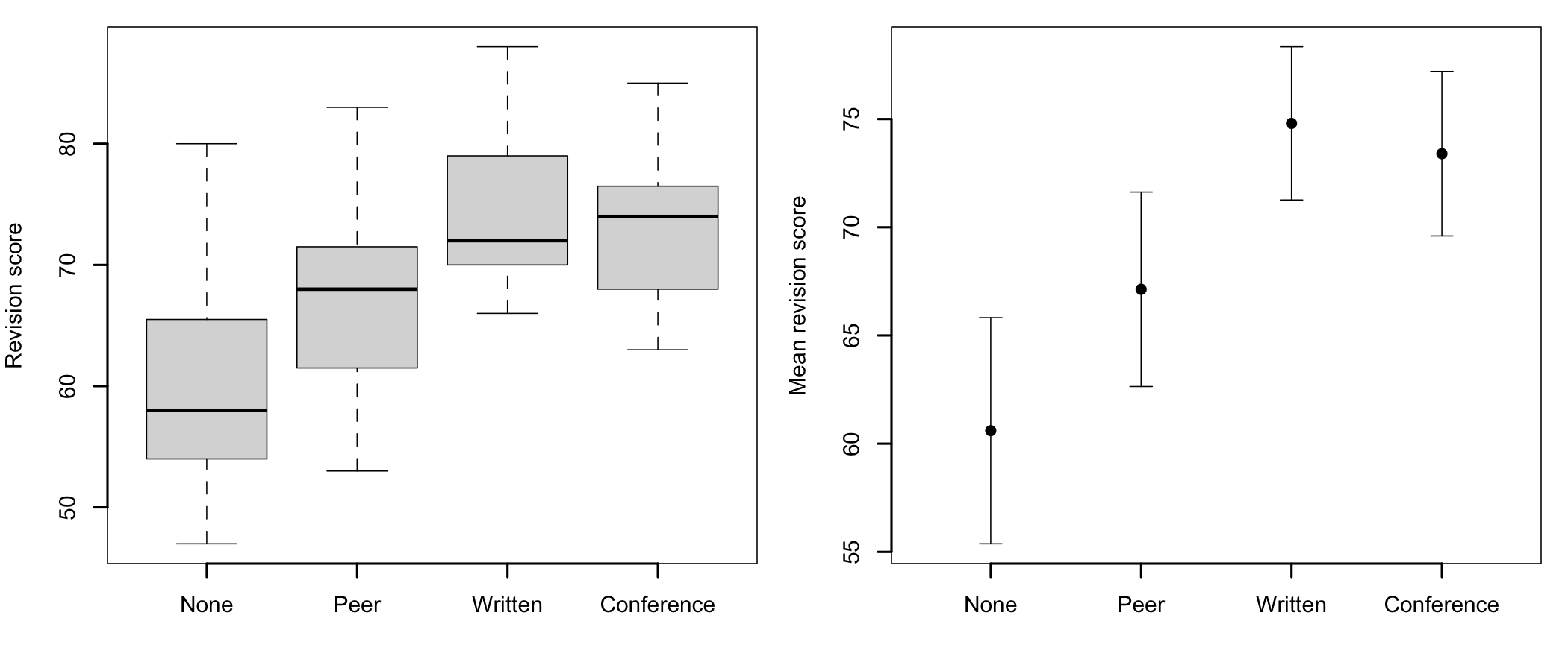
Table 12.4 and Figure 12.1 show that the students who received no feedback obtained the lowest scores (M = 60.60), and those who received feedback from the instructor the highest, in writing (M = 74.80) or in a conference (M = 73.40). The peer feedback group is in between. The confidence intervals of the None group and of the two instructor groups do not overlap, which suggests that these differences will be significant. The spread of the scores is similar in the four groups.
12.4.2 Checking the Assumptions
The independence of observations is supported by the design of the study: the students were randomly assigned to the groups, each student belonged to only one group, and the essays were scored independently.
      None       Peer    Written Conference
 0.3777446  0.9866402  0.3123496  0.6398369
Levene's Test for Homogeneity of Variance (center = mean)
Df F value Pr(>F)
group 3 0.6994 0.5564
56 - Normality. The Shapiro-Wilk test is not significant in any of the four groups (p-values between .312 and .987). There is no evidence of a departure from normality in any group.
- Homogeneity of variances. Levene’s test is not significant, F(3, 56) = 0.70, p = .556. The null hypothesis that the variances are equal cannot be rejected1010 The largest standard deviation (9.43) is also less than twice the smallest one (6.39), a common rule of thumb for the F test..
10 The largest standard deviation (9.43) is also less than twice the smallest one (6.39), a common rule of thumb for the F test.
All assumptions are met, so we can proceed with the analysis.
12.4.3 The ANOVA Test
Before running the test, let’s compute the sums of squares by hand. The grand mean of the revision scores is 68.98. The model sum of squares compares the four group means with it:
SS_{M} = \sum n_k(\bar{Y}_k - \bar{Y})^2 = 15(60.60 - 68.98)^2 + \dots + 15(73.40 - 68.98)^2 = 1905.65
The residual sum of squares, computed from the distance of each score to the mean of its own group, is SS_{R} = 3399.33. Dividing each by its degrees of freedom:
F = \frac{SS_{M} / (k - 1)}{SS_{R} / (N - k)} = \frac{1905.65 / 3}{3399.33 / 56} = \frac{635.22}{60.70} = 10.46
The ANOVA output shows the same values:
            Df Sum Sq Mean Sq F value   Pr(>F)
feedback     3   1906   635.2   10.46 1.45e-05 ***
Residuals   56   3399    60.7
---
Signif. codes:  0 '***' 0.001 '**' 0.01 '*' 0.05 '.' 0.1 ' ' 1
Decision. With F(3, 56) = 10.46, p < .001, the p-value is smaller than \alpha = .05. The null hypothesis is rejected and the alternative hypothesis accepted: the mean revision scores are not the same for all kinds of feedback.
Effect size. \eta^{2} = 1905.65 / 5304.98 = 0.36: the kind of feedback accounts for about 36% of the variance in the revision scores, a large effect. The less biased estimate, \omega^{2} = 0.32, is somewhat smaller, but still indicates a large effect.
12.4.4 The Same Analysis as a Regression
Let’s now fit the same data with a regression model. The four groups are coded as three dummy variables, with the first group, None, as the reference group:
Call:
lm(formula = score ~ feedback, data = fb)

Residuals:
     Min       1Q   Median       3Q      Max
-14.1333  -5.6500  -0.3667   4.6000  19.4000

Coefficients:
                   Estimate Std. Error t value Pr(>|t|)
(Intercept)          60.600      2.012  30.124  < 2e-16 ***
feedbackPeer          6.533      2.845   2.296   0.0254 *
feedbackWritten      14.200      2.845   4.991 6.18e-06 ***
feedbackConference   12.800      2.845   4.499 3.49e-05 ***
---
Signif. codes:  0 '***' 0.001 '**' 0.01 '*' 0.05 '.' 0.1 ' ' 1

Residual standard error: 7.791 on 56 degrees of freedom
Multiple R-squared:  0.3592,    Adjusted R-squared:  0.3249
F-statistic: 10.46 on 3 and 56 DF,  p-value: 1.446e-05
The last line of the output shows the same F test as the ANOVA, F(3, 56) = 10.46, and the R^2 of the model (0.36) is the \eta^{2} computed above. The coefficients describe the group means:
- The intercept, 60.60, is the mean of the reference group, None;
- Each of the other coefficients is the difference between a group mean and the mean of the None group1111 For example, the students who received written feedback scored, on average, 14.20 points more than those who received no feedback (74.80 - 60.60)..
11 For example, the students who received written feedback scored, on average, 14.20 points more than those who received no feedback (74.80 - 60.60).
The t-Tests of the coefficients compare each kind of feedback with no feedback. They answer some of the questions we may have about the groups, but not all of them. The regression does not compare, for example, written feedback with a conference. Answering such questions is the role of the follow-up procedures discussed next.
12.5 Following Up a Significant F
A significant F tells us that at least one group mean differs from the others, but not which one. There are two ways to find out:
- Planned contrasts, when the researcher has specific hypotheses about the groups before collecting the data. They test only these hypotheses, which keeps the number of tests small. Whether to correct \alpha for them is decided, and reported, before the data is collected1212 Planning protects against choosing the comparisons after seeing the data, but each planned contrast still carries its own risk of a Type I error.;
12 Planning protects against choosing the comparisons after seeing the data, but each planned contrast still carries its own risk of a Type I error.
- Post hoc tests, when there are no specific hypotheses and all pairs of groups are compared. They correct for the number of comparisons to keep the familywise error rate at \alpha.
12.5.1 Planned Contrasts
A contrast compares one set of groups with another set by giving each group a weight. The groups on one side of the comparison receive positive weights and the groups on the other side negative weights. Groups left out of a comparison receive a weight of zero. The contrast is the weighted sum of the group means:
\psi = \sum w_k \bar{Y}_k
The weights are chosen following a few rules:
- The weights of a contrast add up to zero1313 This makes the contrast equal to zero when the two sides of the comparison have the same mean, which is what H0 states.;
13 This makes the contrast equal to zero when the two sides of the comparison have the same mean, which is what H0 states.
- With k groups, there are at most k - 1 independent contrasts;
- The contrasts should be orthogonal (independent of each other): the products of their weights, added up across the groups, must be zero for each pair of contrasts.
Orthogonal contrasts divide the model sum of squares into separate, non-overlapping parts, one for each question asked. For the feedback study, the instructor had three questions before the study started:
- C1: Does feedback help at all? No feedback against the three kinds of feedback;
- C2: Is feedback from the instructor better than feedback from peers? Peer feedback against the two instructor groups;
- C3: Does it matter how the instructor gives the feedback? Written comments against a conference.
| None | Peer | Written | Conference | |
|---|---|---|---|---|
| C1 | -3 | 1 | 1 | 1 |
| C2 | 0 | -2 | 1 | 1 |
| C3 | 0 | 0 | -1 | 1 |
The weights in each row of Table 12.5 add up to zero, and the contrasts are orthogonal1414 For C1 and C2, for example, (-3)(0) + (1)(-2) + (1)(1) + (1)(1) = 0, and the same is true for the other two pairs..
14 For C1 and C2, for example, (-3)(0) + (1)(-2) + (1)(1) + (1)(1) = 0, and the same is true for the other two pairs.
C1 C2 C3
 0  0  0
C1 C2 C3
C1 12 0 0
C2 0 6 0
C3 0 0 2Hypotheses. Each contrast has its own pair of hypotheses. For C1, for example, H0: \psi_{1} = 0, the mean of the three feedback groups is equal to the mean of the group without feedback, and H1: \psi_{1} \neq 0. The hypotheses of C2 and C3 are stated the same way.
Decision criteria. The three contrasts are orthogonal and were planned before the study, and each is tested at \alpha = .05, two-tailed, as decided in advance1515 Each contrast still has its own risk of a Type I error, so the chance of at least one among the three is close to .14. A researcher who wants to keep it at .05 tests each contrast at \alpha = .05 / 3 instead.. A contrast is tested with a t-Test that uses MS_{R}, the error term of the ANOVA, with 56 degrees of freedom.
15 Each contrast still has its own risk of a Type I error, so the chance of at least one among the three is close to .14. A researcher who wants to keep it at .05 tests each contrast at \alpha = .05 / 3 instead.
Call:
aov(formula = score ~ feedback, data = fb)

Residuals:
     Min       1Q   Median       3Q      Max
-14.1333  -5.6500  -0.3667   4.6000  19.4000

Coefficients:
            Estimate Std. Error t value Pr(>|t|)
(Intercept)  68.9833     1.0058  68.583  < 2e-16 ***
feedbackC1    2.7944     0.5807   4.812 1.17e-05 ***
feedbackC2    2.3222     0.8213   2.828  0.00649 **
feedbackC3   -0.7000     1.4225  -0.492  0.62457
---
Signif. codes:  0 '***' 0.001 '**' 0.01 '*' 0.05 '.' 0.1 ' ' 1

Residual standard error: 7.791 on 56 degrees of freedom
Multiple R-squared:  0.3592,    Adjusted R-squared:  0.3249
F-statistic: 10.46 on 3 and 56 DF,  p-value: 1.446e-05
The results of the three contrasts1616 Rows feedback1 to feedback3 of the output. can be translated back into differences between means:
16 Rows feedback1 to feedback3 of the output.
- C1: The three feedback groups scored, on average, 11.18 points more than the group without feedback, t(56) = 4.81, p < .001. Feedback helps;
- C2: The two instructor groups scored, on average, 6.97 points more than the peer feedback group, t(56) = 2.83, p = .006. Feedback from the instructor is better than feedback from peers;
- C3: The conference group scored 1.40 points less than the written feedback group, a difference that is not significant, t(56) = -0.49, p = .625. No difference was found between the two ways the instructor gave feedback.
Decision. H0 is rejected for C1 and C2, and cannot be rejected for C3.
The third result has a practical meaning for the instructor. A conference takes much more of the instructor’s time than written comments, and the data does not show that it brings better results.
12.5.2 Post Hoc Tests
When there are no specific hypotheses, all pairs of groups are compared. With four groups there are six comparisons, so the p-values must be corrected. Two of the most common procedures are:
- Tukey’s HSD (Honestly Significant Difference), designed for comparing all pairs of means. It works best when the groups have the same size and the variances are equal;
- The Bonferroni correction, which divides \alpha by the number of comparisons1717 Equivalently, each p-value can be multiplied by the number of comparisons and compared with \alpha.. It can be used with any set of comparisons, but it is conservative: the more comparisons, the harder it becomes to find a difference.
17 Equivalently, each p-value can be multiplied by the number of comparisons and compared with \alpha.
  Tukey multiple comparisons of means
    95% family-wise confidence level

Fit: aov(formula = score ~ feedback, data = fb)

$feedback
                        diff        lwr       upr     p adj
Peer-None           6.533333 -0.9997320 14.066399 0.1110941
Written-None       14.200000  6.6669347 21.733065 0.0000360
Conference-None    12.800000  5.2669347 20.333065 0.0002001
Written-Peer        7.666667  0.1336013 15.199732 0.0446019
Conference-Peer     6.266667 -1.2663987 13.799732 0.1350243
Conference-Written -1.400000 -8.9330653  6.133065 0.9605384
Decision criteria. A pair of groups differs significantly if its adjusted p-value is smaller than \alpha = .05, or, equivalently, if its 95% confidence interval does not include zero1818 In the output, the adjusted p-value is in column p adj, and the confidence interval in columns lwr and upr..
18 In the output, the adjusted p-value is in column p adj, and the confidence interval in columns lwr and upr.
Decision. The Tukey HSD test shows that the students who received written feedback (p < .001) or a conference (p < .001) scored higher than those who received no feedback. The written feedback group also scored higher than the peer feedback group (p = .045). None of the other differences is significant. Peer feedback, in particular, does not differ significantly from no feedback (p = .111).
Let’s compare these results with the Bonferroni correction:
    Pairwise comparisons using t tests with pooled SD

data:  fb$score and fb$feedback

           None    Peer    Written
Peer       0.15247 -       -
Written    3.7e-05 0.05567 -
Conference 0.00021 0.19047 1.00000

P value adjustment method: bonferroni
The two procedures agree on the differences between the None group and the two instructor groups. The difference between the written feedback and the peer feedback groups, however, is no longer significant with the Bonferroni correction (p = .056). This is the price of a conservative correction: the more comparisons are corrected for, the larger a difference must be to reach significance. A result that is significant with one procedure and not with the other, as here, is a borderline result and should be reported with caution.
Of note is the fact that the post hoc tests and the planned contrasts answer different questions, and their results are not directly comparable. The contrast C2, for example, compares the peer feedback group with the two instructor groups together, which is a more powerful test than comparing it with each of them separately.
Which procedure to use? Planned contrasts, when the hypotheses are known before the study, because they test exactly the questions asked and keep the full power of the analysis. Tukey’s HSD, when all pairs of groups are of interest and the groups have similar sizes and variances. The Bonferroni correction, when only a few comparisons are of interest. With unequal variances, the Games-Howell procedure is preferred.
12.6 When the Variances Are Not Equal: Welch’s ANOVA
At a glance
- Use instead of
- The one-way ANOVA, when the variances of the groups are not equal, especially when the groups also differ in size
- Question
- Do the means of two or more independent groups differ?
- Design
- Two or more independent groups, one measurement of each participant
- Dependent variable
- Interval or ratio
- Independent variable
- Nominal, two or more levels
- Assumptions
-
- Independent observations: each participant belongs to one group only
- DV normally distributed in each group
- Null hypothesis
- All population means are equal
- Test statistic
- F, with degrees of freedom adjusted for the unequal variances
- Effect size
- As for the one-way ANOVA
- Include in the write-up
-
- Levene’s test, as the reason for Welch’s version
- F(df1, df2) = …, p = …, with the second df not a whole number
When the variances of the groups are not equal, especially when the groups also differ in size, Welch’s ANOVA adjusts the F test and its degrees of freedom for the unequal variances, the same way Welch’s t-Test does for two groups. In our data the variances are equal, and the Welch test leads to the same conclusion as the ordinary ANOVA:
    One-way analysis of means (not assuming equal variances)

data:  score and feedback
F = 9.1265, num df = 3.000, denom df = 30.833, p-value = 0.0001788
The Welch test confirms the result, F(3, 30.83) = 9.13, p < .0011919 Note that the second number of degrees of freedom is no longer a whole number..
19 Note that the second number of degrees of freedom is no longer a whole number.
12.7 The Kruskal-Wallis Test
At a glance
- Use instead of
- The one-way ANOVA, when the DV is ordinal or clearly not normal in a small sample
- Question
- Do the scores of one or more of several independent groups tend to be higher or lower?
- Design
- Two or more independent groups, one measurement of each participant
- Dependent variable
- Ordinal, interval, or ratio
- Independent variable
- Nominal, two or more levels
- Assumptions
-
- Independent observations: each participant belongs to one group only
- Null hypothesis
- The scores of all groups come from the same distribution
- Test statistic
- H, compared with a chi-square distribution with k - 1 degrees of freedom
- Effect size
- \varepsilon^{2} = H / (N - 1), read like \eta^{2}
- Include in the write-up
-
- The size and median of each group
- Why the rank-based test was used
- H(df) = …, p = …, and \varepsilon^{2}
- The pairwise Mann-Whitney tests, with a Bonferroni correction
The Kruskal-Wallis test is the rank-based alternative to the one-way ANOVA, used when the dependent variable is ordinal or when it is clearly not normally distributed. All scores are ranked together, from the smallest to the largest, regardless of the group they belong to, and the test compares the mean ranks of the groups. It extends the Mann-Whitney U test2020 Also known as the Wilcoxon rank-sum test. to three or more groups, the same way the ANOVA extends the independent samples t-Test. Let’s run it on the revision scores.
20 Also known as the Wilcoxon rank-sum test.
Hypotheses.
- Null hypothesis (H0): In the population, the revision scores of the four feedback groups have the same distribution.
- Alternative hypothesis (H1): In the population, the scores of at least one group tend to be higher or lower than the scores of the others.
Decision criteria. The significance level is set at \alpha = .05. The test statistic, H, follows a chi-square distribution with k - 1 degrees of freedom, where k is the number of groups. H0 is rejected if the p-value is smaller than \alpha. The effect size is epsilon squared, \varepsilon^{2} = H / (N - 1), read with the same guidelines as \eta^{2}.
    Kruskal-Wallis rank sum test

data:  score by feedback
Kruskal-Wallis chi-squared = 20.063, df = 3, p-value = 0.0001647
Decision. With H(3) = 20.06, p < .001, H0 is rejected: the revision scores differ between the feedback groups. The Kruskal-Wallis test leads to the same conclusion as the ANOVA. A significant result is followed by pairwise comparisons of the groups with the Mann-Whitney U test, with a Bonferroni correction.
Effect size. \varepsilon^{2} = 0.34.
When the assumptions of the ANOVA are met, as in this study, the ANOVA is preferred, because it has more power to detect a difference.
A Kruskal-Wallis test compared the revision scores of 60 students randomly assigned to four kinds of feedback. The scores differed significantly between the groups, H(3) = 20.06, p < .001, ε2 = .34, with median scores of 58.0 (none), 68.0 (peer), 72.0 (written), 74.0 (conference).
12.8 Reporting the Results
For reporting, the output should be converted to the format of the publication venue. The American Psychological Association (APA) Publication Manual, for example, recommends the table format shown in Table 12.6.
| Source | df | SS | MS | F | p | ω2 |
|---|---|---|---|---|---|---|
| Feedback | 3 | 1905.65 | 635.22 | 10.46 | < .001 | .32 |
| Residuals | 56 | 3399.33 | 60.70 | |||
| Total | 59 | 5304.98 |
Here is an example of how to write up the results in a publication.
A one-way ANOVA compared the revision scores of 60 students randomly assigned to four kinds of feedback on their first draft. The scores did not depart significantly from normality in any group (Shapiro-Wilk p-values between .312 and .987), and the variances were equal (Levene’s test p = .556). The kind of feedback had a significant effect on the revision scores, F(3, 56) = 10.46, p < .001, ω2 = .32. Planned contrasts showed that the students who received feedback scored higher than those who did not (M = 71.78 vs. M = 60.60), t(56) = 4.81, p < .001, and that feedback from the instructor led to higher scores than feedback from peers (M = 74.10 vs. M = 67.13), t(56) = 2.83, p = .006. Written comments (M = 74.80, SD = 6.39) and conferences (M = 73.40, SD = 6.86) did not differ significantly, t(56) = -0.49, p = .625.
12.9 Summary
The one-way ANOVA compares the means of two or more groups with a single test, which keeps the risk of a Type I error at \alpha. It does so by comparing the variability between the groups with the variability within them. The ANOVA is a regression with a categorical independent variable, and its effect size, \eta^{2}, is the R^2 of that regression.
A significant F says only that the groups differ. Planned contrasts test the specific questions the researcher had before the study, while post hoc tests compare all pairs of groups when there are no such questions. In the feedback study, the contrasts showed that feedback helps, that feedback from the instructor helps more than feedback from peers, and that no difference was found between written comments and a conference. Not finding a difference does not show that the two are equal. Showing that requires an equivalence test.
Of note is the fact that the conclusions can be read as causal only because the students were randomly assigned to the groups. With existing groups, such as students who chose a kind of feedback themselves, the same analysis would show that the groups differ, but not why2121 See A Few Words About Causality..
21 See A Few Words About Causality.