6 Sample Size
A sample is a subset of a population selected to represent the entire population in a study. It is used because while the study is interested in learning more about the population, it may not always be feasible to study every member of that population. The reasons can be, for example, unfeasible incurred costs61 For example in the form of time and money. or, it may just be impossible due to geographical distribution or availability.
6.1 Factors Affecting the Size of the Sample
For any study, the sample size depends on a few elements:
- Level of significance (what is acceptable as an error rate). This is the p-value, such as 95% (\(\alpha\) = 0.05) which indicates the researcher’s readiness to accept a certain probability that the obtained result is due to chance and not to the intervention or researcher’s intention.
- Power, discussed in the context of Type II error, the failure to detect a difference when one doesn’t exist, or the chance of false negatives. The power of the study increases with the decrease in the chance of committing a Type II error. Usually 80% is an acceptable level for the power of a study. It means that the researcher is accepting the study misses a real difference in one in five times. For more strict studies, power can be increased to 90% or more.
- Expected effect size, represents the difference between a variable’s value in one groups and its value in another group. It is inversely proportional with the sample size. There is no formula to determine the effect size. Most often is determined based on prior studies reported in the literature.
- Effect prevalence in the population, estimated from previous studies.
- Population standard deviation, a measure of dispersibility.
When estimating sample size a researcher should consider other elements as well, such as administrative issues, costs, possible participant response rate, and so forth. Each study should be considered from all angles and all potential elements that could participate in determining the sample should be studied carefully.
6.2 Methods of Determining the Sample Size
A cursory review of the literature shows that sample size can be determined in many ways using formulas and/or tables and that there is no universal “formula” for sample size calculations. Each of the methods has a recommended use.
For example, an approach to make a rough determination of a sample size for an experimental design using effect size and power was discussed in the Controlling Power Through Sample Size section. You will also find many sample size calculators available online, many of them based on Cochran’s Sample Size Formula.
6.2.1 Cochran’s Sample Size Formula
Used to compute an ideal sample size for a desired level of precision, it is recommended to be used for studies with infinite populations (Cochran 1977Cochran, W.G. 1977. Sampling Techniques. 3rd ed. New York: John Wiley & Sons.).
\(n_{0}=\dfrac{z^{2}\cdot p\cdot(1-p)}{e^{2}}\)
e: desired level of precision, the margin of error
p: the fraction of the population (as percentage) that displays the attribute
z: the z-value, extracted from a z-table62 The entry for z in a z-table represents the area under the normal distribution curve to the left of z (Figure 6.1)..
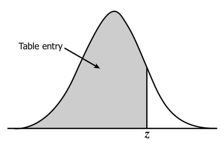 Figure 6.1: Area represented by the z-value.
Let’s consider an example. Think of a study of students in a large university campus for which we don’t know the campus size63 For example a large campus may have 10 - 15 K students. We are interested in finding the percentage of students who eat lunch at the campus dinner halls but we do not have insider information. The question is how many students would we need to ask that question to be able to determine, with reasonable confidence, what percentage of students conform to the sought behavior. Given the lack of information we start by considering that 50% of the students eat lunch at the school dining halls, which provides the largest variability. Then we consider a 95% confidence level (leading to an \(\alpha\)=0.05) and a ±5% precision. From the z-tables, the value for z is 1.96. Therefore, the theoretical sample would be:
\(n_{0}=\dfrac{1.96^{2}\cdot0.5\cdot(1-0.5)}{0.05^{2}}=384.16\approx385\)
How to find the value of z from a z-table. The procedure is:
- Convert the confidence level from percent form to decimal form as value between 0 and 1. (95% \(\rightarrow\) 0.95)
- Subtract the value from 1 and divide by 2 to find out how much is half (1 - 0.95 = 0.05; 0.05/2 = 0.025)
- Add the value from 2) to the value from 1) (0.95 + 0.025 = 0.975)
- Look for the value obtained in step 3) in table values. In Table 6.1 the value sits at the intersection of row labeled 1.9 and column labeled 0.06.
- Determine the value of z by adding the value for the column with the value for the row obtained in step 4 (1.9 + 0.06 = 1.96).
6.2.2 Cochran’s Modified Formula for Finite Populations
A slightly modified formula can be used if the size of the population is known.
\(n=\dfrac{n_{0}}{1+\dfrac{n_{0}-1}{N}}\)
n0: Cochran’s sample size computed using the formula for ideal sample size;
N: the size of the population64 The sample size is dependent on the size of the population until the population reaches about 40-50 K, after which the increase is almost none. Therefore, if the estimated population is this large or larger, the theoretical sample size, as computed for an unknown population, is about equal to the one generated by the modified formula..
As an example, let’s look at the same problem as before but for a much smaller campus of N = 600 students. While we can still use the theoretical sample of 385 participants computed before, do we need to? The necessary sample size may be smaller.
\(n=\dfrac{385}{1+\dfrac{385-1}{600}}=234.76\approx235\)
The result of this computation indicates that for smaller populations the number of subjects (sample size) can be smaller (235 vs. 385) for the researchers to be reasonably confident of the findings.
6.2.3 Yamane’s Simplified Formula for Sample Size
To make it simpler to compute the sample size without over estimating it when the population is known Yamane (1967) proposed the following formula:
\(n=\dfrac{N}{1+N\cdot e^{2}}\)
N - population size
e - level of precision
Using the same example as before, Yamane’s formula would suggest a sample size of 240 subjects for a student population of 600.
\(n=\dfrac{600}{1+600\cdot0.05^{2}}=240\)
Table 6.1: z-table
| 0.00 | 0.01 | 0.02 | 0.03 | 0.04 | 0.05 | 0.06 | 0.07 | 0.08 | 0.09 | |
|---|---|---|---|---|---|---|---|---|---|---|
| 0.0 | 0.5000 | 0.5040 | 0.5080 | 0.5120 | 0.5160 | 0.5199 | 0.5239 | 0.5279 | 0.5319 | 0.5359 |
| 0.1 | 0.5398 | 0.5438 | 0.5478 | 0.5517 | 0.5557 | 0.5596 | 0.5636 | 0.5675 | 0.5714 | 0.5753 |
| 0.2 | 0.5793 | 0.5832 | 0.5871 | 0.5910 | 0.5948 | 0.5987 | 0.6026 | 0.6064 | 0.6103 | 0.6141 |
| 0.3 | 0.6179 | 0.6217 | 0.6255 | 0.6293 | 0.6331 | 0.6368 | 0.6406 | 0.6443 | 0.6480 | 0.6517 |
| 0.4 | 0.6554 | 0.6591 | 0.6628 | 0.6664 | 0.6700 | 0.6736 | 0.6772 | 0.6808 | 0.6844 | 0.6879 |
| 0.5 | 0.6915 | 0.6950 | 0.6985 | 0.7019 | 0.7054 | 0.7088 | 0.7123 | 0.7157 | 0.7190 | 0.7224 |
| 0.6 | 0.7257 | 0.7291 | 0.7324 | 0.7357 | 0.7389 | 0.7422 | 0.7454 | 0.7486 | 0.7517 | 0.7549 |
| 0.7 | 0.7580 | 0.7611 | 0.7642 | 0.7673 | 0.7704 | 0.7734 | 0.7764 | 0.7794 | 0.7823 | 0.7852 |
| 0.8 | 0.7881 | 0.7910 | 0.7939 | 0.7967 | 0.7995 | 0.8023 | 0.8051 | 0.8078 | 0.8106 | 0.8133 |
| 0.9 | 0.8159 | 0.8186 | 0.8212 | 0.8238 | 0.8264 | 0.8289 | 0.8315 | 0.8340 | 0.8365 | 0.8389 |
| 1.0 | 0.8413 | 0.8438 | 0.8461 | 0.8485 | 0.8508 | 0.8531 | 0.8554 | 0.8577 | 0.8599 | 0.8621 |
| 1.1 | 0.8643 | 0.8665 | 0.8686 | 0.8708 | 0.8729 | 0.8749 | 0.8770 | 0.8790 | 0.8810 | 0.8830 |
| 1.2 | 0.8849 | 0.8869 | 0.8888 | 0.8907 | 0.8925 | 0.8944 | 0.8962 | 0.8980 | 0.8997 | 0.9015 |
| 1.3 | 0.9032 | 0.9049 | 0.9066 | 0.9082 | 0.9099 | 0.9115 | 0.9131 | 0.9147 | 0.9162 | 0.9177 |
| 1.4 | 0.9192 | 0.9207 | 0.9222 | 0.9236 | 0.9251 | 0.9265 | 0.9279 | 0.9292 | 0.9306 | 0.9319 |
| 1.5 | 0.9332 | 0.9345 | 0.9357 | 0.9370 | 0.9382 | 0.9394 | 0.9406 | 0.9418 | 0.9429 | 0.9441 |
| 1.6 | 0.9452 | 0.9463 | 0.9474 | 0.9484 | 0.9495 | 0.9505 | 0.9515 | 0.9525 | 0.9535 | 0.9545 |
| 1.7 | 0.9554 | 0.9564 | 0.9573 | 0.9582 | 0.9591 | 0.9599 | 0.9608 | 0.9616 | 0.9625 | 0.9633 |
| 1.8 | 0.9641 | 0.9649 | 0.9656 | 0.9664 | 0.9671 | 0.9678 | 0.9686 | 0.9693 | 0.9699 | 0.9706 |
| 1.9 | 0.9713 | 0.9719 | 0.9726 | 0.9732 | 0.9738 | 0.9744 | 0.9750 | 0.9756 | 0.9761 | 0.9767 |
| 2.0 | 0.9772 | 0.9778 | 0.9783 | 0.9788 | 0.9793 | 0.9798 | 0.9803 | 0.9808 | 0.9812 | 0.9817 |
| 2.1 | 0.9821 | 0.9826 | 0.9830 | 0.9834 | 0.9838 | 0.9842 | 0.9846 | 0.9850 | 0.9854 | 0.9857 |
| 2.2 | 0.9861 | 0.9864 | 0.9868 | 0.9871 | 0.9875 | 0.9878 | 0.9881 | 0.9884 | 0.9887 | 0.9890 |
| 2.3 | 0.9893 | 0.9896 | 0.9898 | 0.9901 | 0.9904 | 0.9906 | 0.9909 | 0.9911 | 0.9913 | 0.9916 |
| 2.4 | 0.9918 | 0.9920 | 0.9922 | 0.9925 | 0.9927 | 0.9929 | 0.9931 | 0.9932 | 0.9934 | 0.9936 |
| 2.5 | 0.9938 | 0.9940 | 0.9941 | 0.9943 | 0.9945 | 0.9946 | 0.9948 | 0.9949 | 0.9951 | 0.9952 |
| 2.6 | 0.9953 | 0.9955 | 0.9956 | 0.9957 | 0.9959 | 0.9960 | 0.9961 | 0.9962 | 0.9963 | 0.9964 |
| 2.7 | 0.9965 | 0.9966 | 0.9967 | 0.9968 | 0.9969 | 0.9970 | 0.9971 | 0.9972 | 0.9973 | 0.9974 |
| 2.8 | 0.9974 | 0.9975 | 0.9976 | 0.9977 | 0.9977 | 0.9978 | 0.9979 | 0.9979 | 0.9980 | 0.9981 |
| 2.9 | 0.9981 | 0.9982 | 0.9982 | 0.9983 | 0.9984 | 0.9984 | 0.9985 | 0.9985 | 0.9986 | 0.9986 |
| 3.0 | 0.9987 | 0.9987 | 0.9987 | 0.9988 | 0.9988 | 0.9989 | 0.9989 | 0.9989 | 0.9990 | 0.9990 |