8 Normalization, Standardization, and Data Transformation
In statistics the term normalization can have multiple meanings. For example, it can mean to adjust values of variables to be analyzed to a common scale when these variables are measured using different scales. Alternatively, normalization may mean to transform the values of a sample to get it closer to the normal distribution, to fulfill the assumption of normally distributed data underlying many common statistical tests. Or, in other situations, normalization could be an attempt to eliminate the effects of known influences.
Sometimes the term normalization is used interchangeably with the term standardization. While both serve the same general purpose, there is a difference:
- Normalization: intended to scale a variable to a range of values between 0 and 1;
- Standardization (e.g., z-score): intended to transform a variable to have its mean = 0 and SD78 Standard Deviation = 1.
Some of the processes that fall under the concept of normalization may be called data transformation79 IMPORTANT: A transformed value, such as a log of the data, has little informational value when interpreted and presented. Therefore the once the analysis has been performed, when discussing the findings, that data should be converted back to its original format by applying the reverse sequence of formulae that was used to transform it in the first place.. While all this may be confusing, the process always involves a purposeful conversion of the data of a data set from its current format to a different format. In most situations, the process also involves eliminating the units of measure with the intent of making the comparison easier.
8.1 Scaling/Rescaling
A very simple process which aims to change the spread of the data and/or the position of the data points. The transformation uses a simple linear equation of the form \(y=a\times x+b\), but leaves unchanged the shape of the distribution or the z-scores80 Because they are calculated as a ratio of the difference between the actual value and the sample’s mean and the sample’s standard deviation. In essence, the z-socre indicates how many standard deviations from the mean the data point is. . It will change the data median, mean (\(\mu\)), and standard deviation (\(\sigma\)).
The more common are:
- Range scaling: change the data from one range to another (magnification or reduction)81 Often times done to bring the variables in an analysis to the same scale.;
- Mean centering: changes the data by subtracting the mean of the sample from each data point, resulting in a shifting of the data towards the mean, effectively making the mean of the scaled data set to be 082 Often done to center the analysis on the variation part of the data rather than, for example, a center tendency value.;
- Standardization: is intended to make data samples comparable. The process does not change the shape of the distribution, only the mean and the standard deviation. The most common method is the z-transform used to convert the data to z-scores. Also called auto-scaling, the z-transform makes the data comparable by transforming observed data into multiples of its standard deviation (SD). The mean of the z-transformed sample is equal to 0. If the original distribution of the data is normal, the transformed data will also follow a normal distribution with a mean of 0 and a standard deviation of 1 (Figure 8.1).
Figure 8.1: z-transformation of data

8.2 Distribution Normalization
There are many real world processes that generate data that do not follow the normal, Gaussian, distribution. Previous sections already discussed how to determine if the data are normally distributed or not. Non-normal data usually fits in one of two categories: 1) follows a different distribution or 2) is a mixture of distributions and data generation processes.
For the data that follows a known distribution83 E.g., binomial, log-normal, exponential, etc., one can either identify the theoretical distribution it follows and analyze the data using tests appropriate for that distribution or somehow transform it to a normal distribution before analysis and then use tests that assume data distribution to be normal.
Dealing with the 2nd category of non-normal data, which displays a mixture of distributions, is more complicated because few, if any, transformations would be able to deal with all that variability for the entire data set. In this case, the data needs to be studied and refined before analysis. For example, an attempt to break down the data can produce sub-samples or categories for which, individually, the distributions are known or recognizable. In this case, transformations can be applied to each sub-sample or category. If the observed data is produced by multiple processes, such as business data produced by complex work activities, multiple shifts, locations, customers, seasonality, etc., an attempt to review the individual process that produced data points and find a common denominator to transform the data to can sometimes help bring the data close enough to the normal distribution so that analysis is possible84 The process always works better for larger samples..
Some of the common options are:
- Box-Cox transformation: Uses a family of power functions to transform data to a more normal distribution form. The formula used for transformation are simple but computationally intensive. For this reason most statistical analysis packages (e.g., SPSS) offer an option to run Box-Cox transformations on the data set.
- Log transformation: The value of each observation is transformed by applying the base 10 or natural logarithm to the observed value. The reverse process is to raise the values at the power of 10 or e85 For the natural logarithms., depending of what type of logarithm was initially applied. It is especially useful if the original variable follows a log distribution; after transformation the resulted values will be normally distributed.
- Square-root transformation: The value of each observation is transformed by taking its square root. To reverse the process is to square the values. Usually used when the variable is a count of something. If the sample includes negative values, the sample should be first rescaled to have all positive values86 For example by adding a certain amount to each observed value..
- Arcsine transformation: The value of each observation is transformed by taking the arcsine of the square root of the number. The numbers to be transformed should be between 0 and 1. The resulted unit of measure is radians and the resulting range is \(-\pi/2\) to \(\pi/2\). It is usually useful for proportions or ratio type data that ranges between 0 and 1.
Let’s look at an example of a log transformation. The origin and meaning of the data set is irrelevant for this transformation example.
A histogram and qq-plot of the original sample data (Figure 8.2):
Figure 8.2: Original data

A visual inspection of the data shows that it is significantly different from a normal distribution and most likely closer to an exponential distribution. So, let’s do a log transformation of the data. Once the data has been transformed, it becomes normally distributed (Figure 8.3).
Figure 8.3: Log transformed data
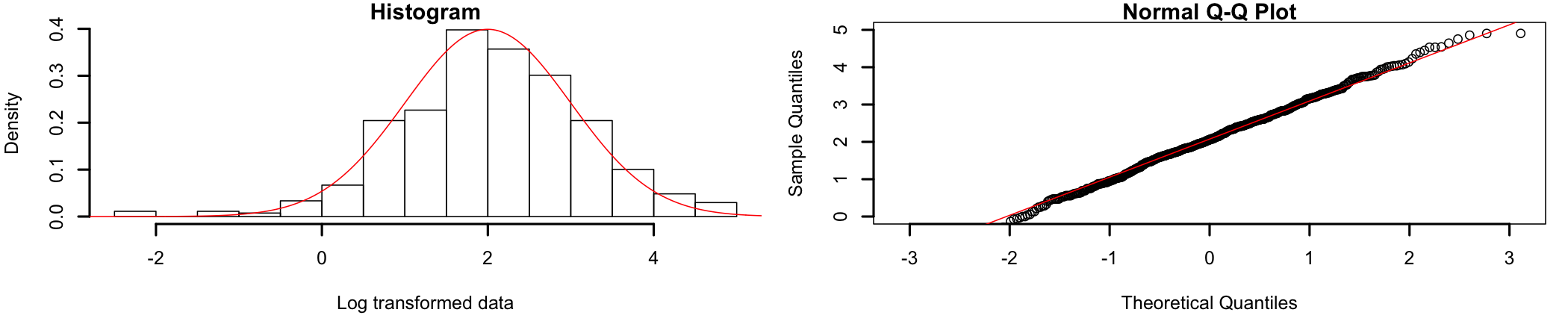
Much better. Now that the assumption of normality is verified (alongside all other assumptions), the analysis can continue.
Once the analysis is completed the data should be transformed back to its original format for interpretation and reporting.