14 Multiple Linear Regression Analysis
Linear Regression is used to study/describe the predictive relationship between one criterion (DV) variable and one or more predictor (IV) variable(s). The procedure can be used to either explore the predictive relationships between a set of variables or to test a causal model. It can be applied when:
- The dependent variable is continuous;
- The independent variable(s) is continuous, discrete or categorical.
It is a highly flexible procedure, especially helpful in non-experimental research in the social sciences field where researchers often deal with naturally occurring variables96 Variables measured as they naturally occur and are not manipulated in any way by the researchers.. The procedure allows researchers to determine if a given set of variables (predictors) is useful in predicting a criterion variable.
The intent of the linear regression analysis is to find the best fitting line of a set of data points. Remember, the simple regression equation is of the form:
\[ Y = a + bX\]
It is the equation representing a straight line in the two dimension plane. In this equation, \(Y\) is the criterion variable (the response), \(X\) is the predictor variable, \(a\) is the intercept97 The value of \(y\) when \(X = 0\), or the point where the line intersects the \(Y\) (vertical) axis., and \(b\) is the slope of the line.
Multiple linear regression expands on the simple linear regression model and attempts to account for how multiple predictors contribute to the value of the criterion variable. In this case the question has the form:
\[Y = a + b_1X+b_2X+...+b_nX\]
The question is still one of straight line98 Using algebra, we can rewrite the equation as: \[Y = a + (b_1 + b_2 + ... + b_n)X\] which is similar to the previous equation (\(b = b_1 + b_2 + ... + b_n\)). The \(b_i\) coefficients represent the contributions of each individual predictor.
Multiple regression allows researchers to:
- Explore the relationship between the criterion variable and the predictor variables as a group and determine whether the relationships is statistically significant;
- Determine how much of the variance of the criterion variable can be accounted for by the predictors, individually and as a group;
- Determine the relative importance of the predictor variables.
Of note is the fact that regression analysis cannot provide strong evidence of a causal relationship between the variables but rather show that the findings are or are not consistent with the causal model under study99 The correlational nature of the data leads to multiple possible ways of interpreting the results.. In case of modeling causal relations, if none of the regression coefficients were found to be significant, the model failed to pass a test100 Alternatively, if significance was observed, the causal model passed an attempt at disconfirmation..
When designing the study researchers may not have sufficient knowledge to determine how the predictors affect the criterion variable. The model they build is their best guess based on their prior knowledge101 Based on existing literature, prior experience, other experiments they have conducted, etc. of the problem they are investigating. For this reason, to find the model that best represents the phenomena, regression analysis offers multiple pathways for conducting the analysis. This example looks at the enter, forward, and backward regression models.
The enter model includes all predictors while the stepwise regression forward and backwards models attempt to reach a more parsimonious (see Occam’s Razor for details) model by reducing the number of predictor variables while attempting to explain as much as possible of the criterion variable. The differences in the quality of the predicted scores can be studied by looking at the three models side by side. A comparative analysis of the forward and backward models will offer the opportunity to validate the results of the analysis when the two methods reach the same solution (regression equation) or if they are very close.
The enter model, as its name suggests, will include all predictors in the regression equation from the beginning. The forward model will enter the variables in the model one by one, starting with the predictor that has the highest order partial correlation with the criterion variable, and then calculating the regression statistics. The process continues by adding the remaining predictor variables, one by one, in descending order of their partial correlations with the dependent variable. This continues as long as the addition of a new predictor variable to the model brings significant102 The goodness of fit of an estimated statistical model is measured by either the Akaike’s Information Criterion (AIC) or the Bayesian Information Criterion (BIC). The lower the value or AIC or BIC is, the better the model is. When the AIC/BIC of two successive models are compared and found significantly different, the model with the better (lower) values is retaind. changes in the model’s predictive power103 The predictive power of the model is reflected in the value of R2.. The backwards model starts with the full model104 The same model as the enter model. and continues by removing predictor variables one by one, in the reverse order of their partial correlation with the criterion variable. The process continues until the updated model does not improve on the previous one.
Prior to the analysis we should familiarize ourselves with the data. Here are a few things to do to better understand what we are working with.
- Check for errors105 E.g., data entry, missing values, etc.;
- Outliers;
- Unusual distributions;
- Clustering or systematic patterns106 If the data groups together in certain ways, forming areas where data is concentrated.;
- Anything else unexpected.
14.1 Assumptions
In regression analysis assumptions are intertwined with the analysis itself. That is, some of the assumptions can only be verified once the model has been defined and after the analysis has been run and the results computed. Regression analysis assumptions are:
- Linear relationship between the predictor (IV) variables and the criterion (DV) variable
- Detected using plots of the residuals107 The residual is the difference between the observed value of the dependent variable and the value predicted by the regression model. The mean of residuals is zero, as is their sum. Residuals help us understand how well the regression line (equation) approximates the data from which it was generated. against each continuous predictor and predictive values;
- The assumption is violated when large or systematic deviations of the fit line are observed around the 0-line108 Representing the mean of the residuals.. A violation is indicative of a non-linear relationship.
- Correct model specification
- Detected by performing the R Squared Change test to determine if adding a variable (given that the theoretical model supports it) to the regression model significantly increases R Square.
- If the R Square Change test is significant, the variable should be included in the regression model. Otherwise, if the test is not significant, do not include the variable.
- No measurement error in the predictor (IV) variables
- Detected by examining the reliability coefficients for the predictor (IV) variables;
- Inadequate reliability if the coefficients are less than .70.
- Homoscedasticity, residuals have constant variance
- Detected by plotting the residuals against each continuous predictor and predicted values;
- Relationship between variability of the residuals and either the predictor (IV) variables or the predicted values indicate heteroscedasticity.
- Residuals are independent, reflecting a clustering or serial dependency problem
- Clustering is detected by using plots of residuals against the grouping/cluster variable using Box Plots;
- The clustering assumption is violated if there is variability in the median value of the residuals in each group;
- Serial dependency is detected by looking at the measure of autocorrelation using the Durbin-Watson test;
- The serial dependency assumption is violated if the Durbin-Watson test results in values less then or greater than 2.
- Clustering is detected by using plots of residuals against the grouping/cluster variable using Box Plots;
- Normal distribution of residuals109 In case of linear regression, a plot of residuals should look as a random cloud of points alongside the regression line. If a pattern is observed in how the residuals are arranged (e.g., they seem to align along a curve), it may be an indication that a non-linear model may be a better fit.
- Detected by using normal probability plots and histogram plots of residuals;
- Non-normal distribution of residuals indicate a violation;
- Residuals that fall far from the straight line indicate a violation.
14.2 The Study
A study was conducted in a Midwestern state in the US to gauge consumers’ interest in purchasing and consuming the different kinds of nuts110 Chestnuts, pecans, and black walnuts. available on the market. The primary focus of the study was to attempt to predict future market behavior based on consumption of, familiarity with, and interest in the product. The data was collected using a survey-type instrument. With the exception of demographic data, the questions used 5-point Likert scales.
For the purpose of this analysis, three variables, defined from the raw dataset, were chosen:
- Interest in buying raw nuts from farmers markets or grocery stores;
- Interest in buying prepared/semi prepared products that contain nuts at farmers markets or from grocery stores;
- Interest in consuming, in restaurants, prepared food that contains nuts;
The questionnaire was freely distributed during a local festival. A number of 232 responses were collected.
14.3 Preliminary Steps
For all quantitative studies is always helpful to familiarize yourself with the data, how it looks, etc. So, let’s look at the first few lines of the dataset111 Due to the large number of variables, only the firs 10 are shown..
Table 14.1: First few rows and variables of the chestnut data set.
| D1.1 | D2.1 | D3.1 | F1.1 | F1.2 | F1.3 | F1.4 | F1.5 | F1.6 | F2.1 |
|---|---|---|---|---|---|---|---|---|---|
| 3 | 4 | 4 | 3 | 4 | 4 | 5 | 4 | 3 | 3 |
| 2 | 3 | 2 | 3 | 5 | 5 | 2 | 2 | 4 | 4 |
| 3 | 5 | 5 | 1 | 1 | 1 | 1 | 1 | 1 | 3 |
| 2 | 2 | 1 | 2 | 3 | 4 | 3 | 3 | 2 | 2 |
| 1 | 1 | 1 | 2 | 5 | 5 | 4 | 5 | 5 | 2 |
| 1 | 1 | 1 | 2 | 2 | 2 | 1 | 1 | 1 | 3 |
14.3.1 Missing Cases
Due to the large sample available, for the purpose of this example, the cases with missing variables were deleted list wise.
14.3.2 Variable Recoding
Table 14.2: Variables included in the analysis
| Name | Type | Value Range | Description |
|---|---|---|---|
| BuyRaw | DV | 3-15 | Interest in buying raw nuts |
| Price | IV | 3-15 | How much the product’s price influences purchase/consumption decision |
| Quality | IV | 3-15 | How much the product’s quality influences purchase/consumption decision |
| Taste | IV | 3-15 | How much the product’s taste influences purchase/consumption decision |
| LocGrown | IV | 3-15 | How much the fact that the product is locally grown influences purchase/consumption decision |
| PrepEase | IV | 3-15 | How much product’s ease of preparation influences purchase/consumption decision |
| Nutrition | IV | 3-15 | How much product’s nutrition factor influences purchase/consumption decision |
The survey was designed to enable a detailed study of the market, for which reason the questions used to collect the data were divided between the three categories of products: chestnuts, pecans, and black walnuts. To capture an overall view of the market the three categories are merged into a single variable. This example analysis will look at the following variables (Table 14.2112 The value of a variable for all the variables listed in Table 14.2 is determined by summing the scores of three questions together. Therefore, if the Likert scale used is from 1 to 5, the minimum value is 3 and the maximum is 15.):
The new variables described in Table 14.2 are computed, using an addition-based model, based on the participants’ responses to survey questions (Table 14.3). Table 14.4 shows a few lines showing the newly created variables.
Table 14.3: Variable recoding
| Variable | Component Questions |
|---|---|
| BuyRaw | D1.1 + D2.1 + D3.1 |
| Price | F1.1 + F2.1 + F3.1 |
| Quality | F1.2 + F2.2 + F3.2 |
| Taste | F1.3 + F2.3 + F3.3 |
| LocGrown | F1.4 + F2.4 + F3.4 |
| PrepEase | F1.5 + F2.5 + F3.5 |
| Nutrition | F1.6 + F2.6 + F3.6 |
Table 14.4: Recoded variables
| BuyRaw | Price | Quality | Taste | LocGrown | PrepEase | Nutrition |
|---|---|---|---|---|---|---|
| 11 | 9 | 12 | 12 | 15 | 10 | 9 |
| 7 | 11 | 13 | 13 | 6 | 6 | 12 |
| 13 | 9 | 11 | 11 | 11 | 11 | 11 |
| 5 | 6 | 9 | 13 | 9 | 9 | 6 |
| 3 | 6 | 15 | 14 | 13 | 15 | 15 |
| 3 | 6 | 6 | 6 | 3 | 3 | 5 |
14.4 Summary Statistics
As a first attempt to discover any possible abnormalities in the data it is always helpful to run summary statistics on the variables in the dataset.
A cursory analysis of the data in Table 14.5 shows that there are no unexpected problems with the data. For example, for all variables the number of included cases is the same (184), meaning that there are no missing cases, the min (3) and max (15) represents the correct range determined by the way the variables were computed (Tables 14.3 and 14.4).
Table 14.5: Summary statistics for the study variables
| vars | n | mean | sd | median | trimmed | mad | min | max | range | skew | kurtosis | se | |
|---|---|---|---|---|---|---|---|---|---|---|---|---|---|
| BuyRaw | 1 | 184 | 9.109 | 3.120 | 9.0 | 9.122 | 2.965 | 3 | 15 | 12 | -0.1058 | -0.5286 | 0.2300 |
| Price | 2 | 184 | 9.277 | 2.591 | 9.0 | 9.324 | 2.965 | 3 | 15 | 12 | -0.1676 | 0.0790 | 0.1910 |
| Quality | 3 | 184 | 11.207 | 2.929 | 12.0 | 11.507 | 2.965 | 3 | 15 | 12 | -0.8162 | 0.3884 | 0.2159 |
| Taste | 4 | 184 | 11.636 | 2.932 | 12.0 | 11.986 | 2.965 | 3 | 15 | 12 | -0.8755 | 0.4133 | 0.2161 |
| LocGrown | 5 | 184 | 9.924 | 3.245 | 10.0 | 10.040 | 2.965 | 3 | 15 | 12 | -0.3064 | -0.5388 | 0.2392 |
| PrepEase | 6 | 184 | 10.114 | 3.034 | 10.0 | 10.250 | 2.965 | 3 | 15 | 12 | -0.4631 | -0.2139 | 0.2237 |
| Nutrition | 7 | 184 | 10.663 | 3.478 | 11.5 | 10.946 | 3.707 | 3 | 15 | 12 | -0.4941 | -0.6215 | 0.2564 |
Before moving forward we need to define the full regression model as the decision to buy as a function of price, quality, taste, growth place, ease of preparation, and nutrition qualities. It can be represented as a linear relationship of the study’s predictors:
\[ \begin{array}{c} BuyRaw'=b_{0}+b_{1}\cdot Price+b_{2}\cdot Quality+b_{3}\cdot Taste\\ +b_{4}\cdot LocGrown+b_{5}\cdot PrepEase+b_{6}\cdot Nutrition \end{array} \]
14.5 Outliers
Let’s look at residuals plot first (Figure 14.1). In this representation an outlier would be a point situated outside the \(\pm3\) interval113 Colored in red or highlighted. represented on the vertical (y) axis. According to this test, only one of the cases is situated close to the -3 limit and could be considered an outlier. Because there are other cases that are relatively close to the limits and because the sample size is sufficiently large, further analysis should be considered to determine if the data point is a real outlier or not. For this purpose further testing will use Mahalanobis distances114 Mahalanobis distance (MD) is the distance between two points in multivariate space. It measures the distance relative to a base or central point considered as an overall mean for multivariate data (centroid). The centroid is a point in multivariate space where the means of all variables intersect..
The histogram in Figure 14.2 suggests that there is at least one outlier in the dataset, indicated by the highlighted bar at the far right of the histogram. While the analysis so far tells us that outliers may exist in the data set, it is not able to help us determine what impact these outliers may have115 Cases that may look like outliers at first sight may not be so after a more in-depth analysis.. Computing Cooks distance116 Cook’s distance is a measure used to estimate the influence of a data point in regression analysis. It measures how much deleting an observation influences the results. Data points with a large value of the computed Cook’s distance are potential outliers and should be subjected to further examination. will provide the means for a closer analysis of potential outliers. Figure 14.3 presents a graphical representation with possible outliers highlighted.
Based on Cook’s distance, the dataset may have three outliers (observations 5, 26, and 110). Considering what we’ve learned so far about the outliers in the dataset, we have two options:
Figure 14.1: Case-wise plot of standardized residuals

Figure 14.2: Histogram of Mahalanobis distances
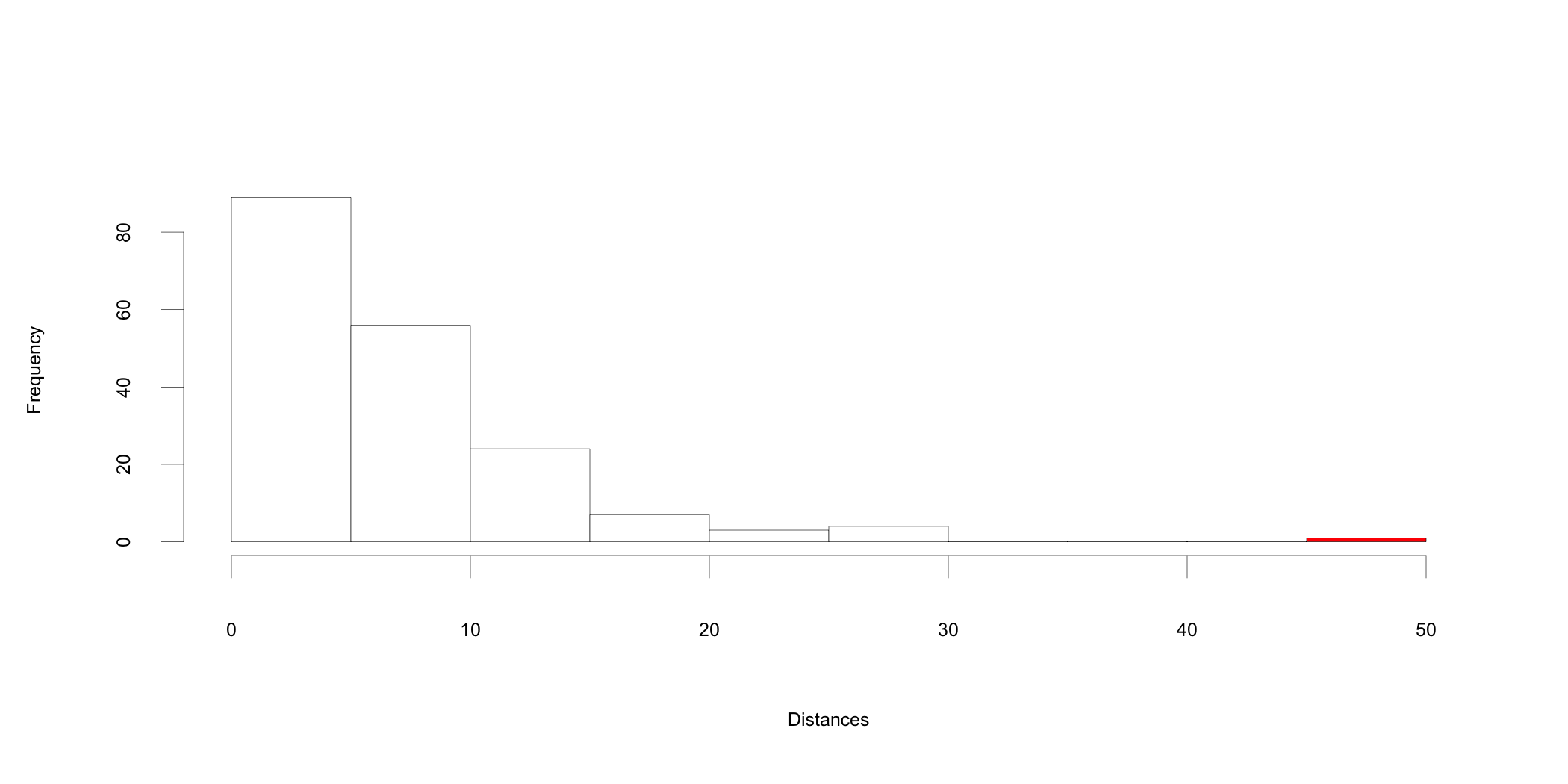
Figure 14.3: Cook’s distance

- Remove the outliers from the dataset and re-run the outlier analysis to determine if the new dataset has more;
- Investigate these outliers further and learn more about their influence and determine what potential leverage they may have on the results of the analysis.
If we have sufficient data points for the analysis117 If the remaining number of records after removing the outliers is larger than the sample size needed for analysis. The sample size is one of the deciding factors in how well the results can be generalized to the population the model attempts to represent., the entire observation or record including the outliers can be removed from the data set. Alternatively, if the removal of outliers reduces sample size too much or if the analysis begins with an undersized sample, the outliers should be analyzed further to determine if they should indeed be removed or if they can be retained thus improving the relevance of the findings to the population118 Removing observations from the dataset may have unwanted effects. For example, when studying opinions, by removing a record showing an extreme, we may unintentionally remove an opinion that may be relevant to the results and affect the outcomes. That is, outliers may be influential observations that have a reason to be kept in the analysis. In addition to numerical analysis, the theory, literature, and previous studies should be used as well to guide the decision..
With this study being used as an example, we will pursue the second option and look further into what leverage outliers may have. For that purpose we can use a scatter plot representation of deleted vs. raw residuals (Figure 14.4). If in the graphical representation all the points, and especially those highlighted so far as outliers, align along the diagonal of the plot area, represented as a line, it can be concluded that none of the points representing potential outliers has a significant leverage and that it may be reasonable to keep them in the dataset.
Figure 14.4: Deleted vs. raw residuals plot

While prior analysis may indicate the existence of potential outliers, leverage analysis suggests their influence is sufficiently weak to warrant including the observations in the analysis.
14.6 Residuals Analysis
Figure 14.5: Normal probability plots

Multiple regression analysis assumes linear relationships between the variables included in the equation and the normal distribution of residuals. When these assumptions are violated, the final conclusion drawn may not be accurate. Normal probability plots are used to test these assumptions (Figure 14.5 left). The grouping of the points close to the straight line119 The representation is a quantile-quantile plot and is interpreted similarly. supports the assumption that the residuals are normally distributed. The same assumption is also supported by the histogram representation of the residuals (Figure 14.5 right).
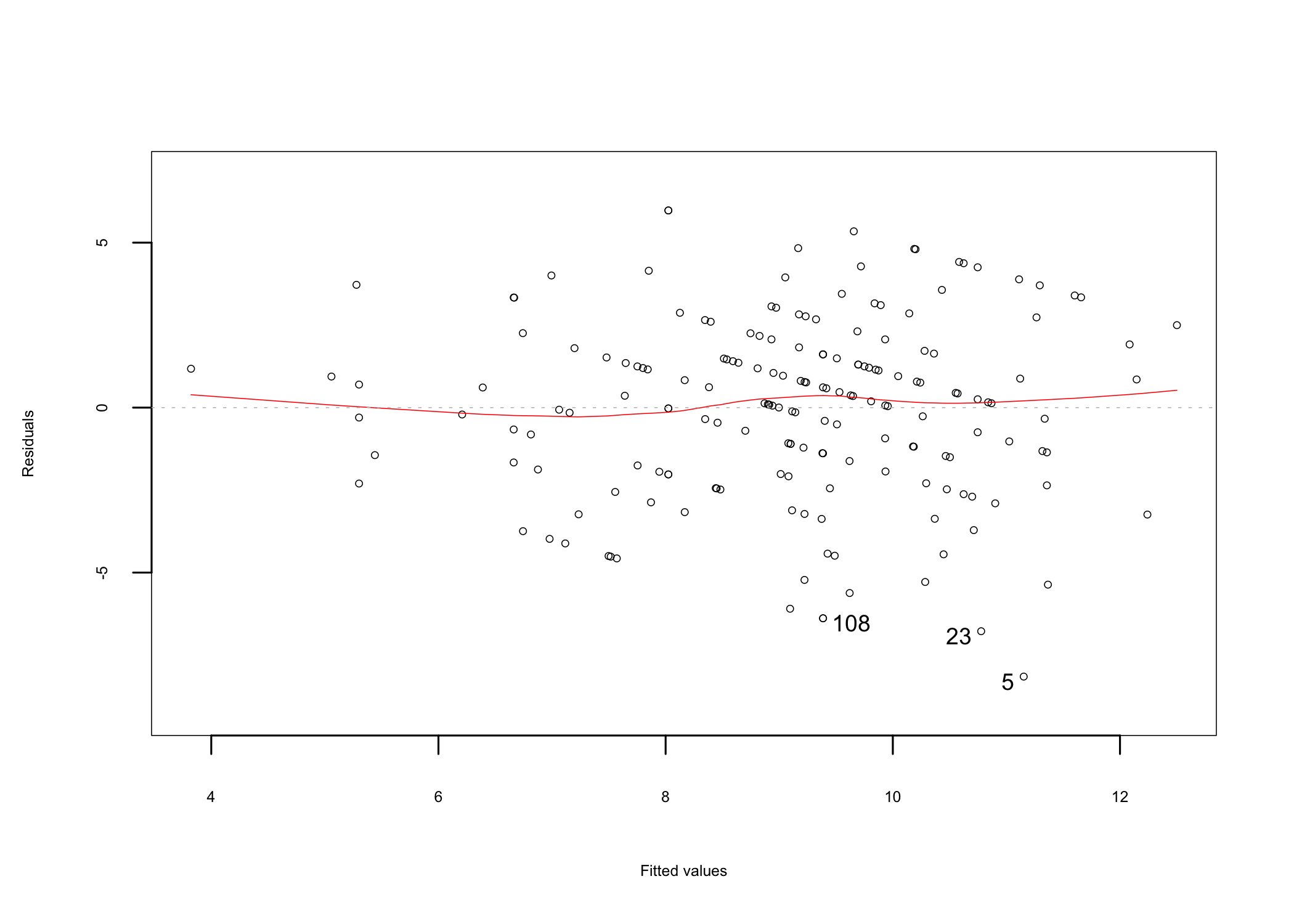
14.7 Linearity
A simple residuals vs fitted plot can be used to test the linearity assumption (Figure 14.6). If linearity is observed, the data points plotted on the graph should resemble a homogeneous cloud around the center line, which should be approximately horizontal at zero. Alternatively, a pattern is indicative of a problem with the linear model. In this analysis, the distribution of the points and the center line (red) suggest that a linear relationship between the criterion and predictor variables can be assumed.
Figure 14.6: Residuals vs. fitted linearity plot
14.8 Enter or Full Model
Up to this point the preliminary analysis of the assumptions has been conducted using the full regression model, which includes all predictor variables. As a reminder, the regression equation for the enter model is120 BuyRaw’ is the estimated value of the criterion variable.:
\[ \begin{array}{c} BuyRaw'=b_{0}+b_{1}\cdot Price+b_{2}\cdot Quality+b_{3}\cdot Taste\\ +b_{4}\cdot LocGrown+b_{5}\cdot PrepEase+b_{6}\cdot Nutrition \end{array} \]
In regression analysis the correlations should be high between the criterion and predictor variables and low between predictor variables. There are multiple ways to look at the correlations between the predictor variables and a wide variety of graphical representations to help the analysis. For example, a visualization of the variable correlations is shown in Figure 14.7.
Figure 14.7: Predictors correlation matrix
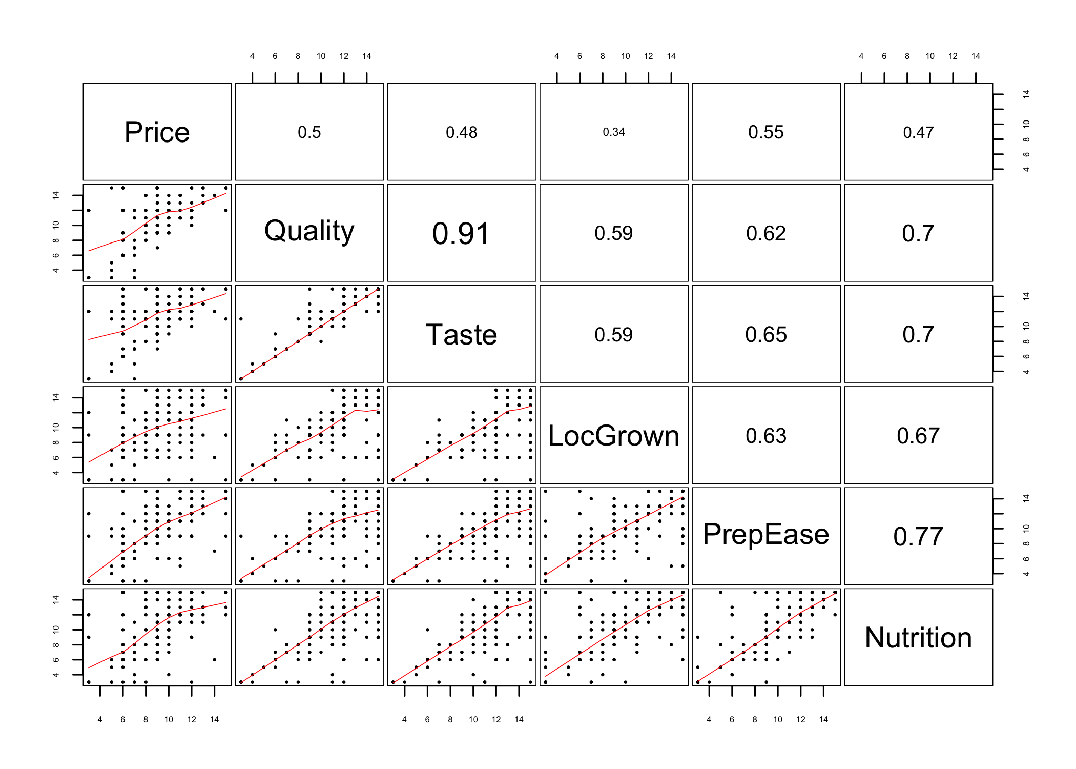
Figure 14.7 shows the predictors on the diagonal, the value of the correlation coefficient between each pair of two predictors above the diagonal, with larger font for higher correlations, and a scatter plot of each pair below the diagonal. The numerical values of the correlation coefficients are fairly easy to interpret. The closer the value is to 1, the higher the correlation is. The closer the value is to 0, the lower the correlation is. Therefore, we are looking to have low values across the board. In this case, quality is highly correlated to taste, as indicated by the value of correlations coefficient of 0.91.
Looking at the scatter plots below the diagonal, we want to see the data points distributed across the plot area rather than forming a pattern. Looking at the same two variables as discussed above, the scatterplot representation shows the points arranged close to and alongside the red diagonal line, forming a diagonal pattern. Other scatter plots may look more distributed, but a closer inspection shows that in some of them the many of the points are concentrated in a pattern along the red diagonal line.
A table representation of the correlations coefficients between the variables in the study (Table 14.6) may be more helpful, especially when it is associated with a table showing the significance levels (Table 14.7) of these correlations.
Table 14.6: Variable correlations
| BuyRaw | Price | Quality | Taste | LocGrown | PrepEase | Nutrition | |
|---|---|---|---|---|---|---|---|
| BuyRaw | 1.00 | 0.18 | 0.47 | 0.41 | 0.33 | 0.25 | 0.38 |
| Price | 0.18 | 1.00 | 0.50 | 0.48 | 0.34 | 0.55 | 0.47 |
| Quality | 0.47 | 0.50 | 1.00 | 0.91 | 0.59 | 0.62 | 0.70 |
| Taste | 0.41 | 0.48 | 0.91 | 1.00 | 0.59 | 0.65 | 0.70 |
| LocGrown | 0.33 | 0.34 | 0.59 | 0.59 | 1.00 | 0.63 | 0.67 |
| PrepEase | 0.25 | 0.55 | 0.62 | 0.65 | 0.63 | 1.00 | 0.77 |
| Nutrition | 0.38 | 0.47 | 0.70 | 0.70 | 0.67 | 0.77 | 1.00 |
The data in Table 14.6 suggests that the higher correlations between the criterion variable BuyRaw and any of the predictor variables is with Quality, at 0.47.
Table 14.7: Significance levels of variable correlations
| BuyRaw | Price | Quality | Taste | LocGrown | PrepEase | Nutrition | |
|---|---|---|---|---|---|---|---|
| BuyRaw | NA | 0.015 | 0 | 0 | 0 | 0.001 | 0 |
| Price | 0.015 | NA | 0 | 0 | 0 | 0.000 | 0 |
| Quality | 0.000 | 0.000 | NA | 0 | 0 | 0.000 | 0 |
| Taste | 0.000 | 0.000 | 0 | NA | 0 | 0.000 | 0 |
| LocGrown | 0.000 | 0.000 | 0 | 0 | NA | 0.000 | 0 |
| PrepEase | 0.001 | 0.000 | 0 | 0 | 0 | NA | 0 |
| Nutrition | 0.000 | 0.000 | 0 | 0 | 0 | 0.000 | NA |
Looking at the correlations between the predictor variables (Table 14.6) the the associated p-values (Table 14.7) it appears that this data set has a problem. The correlations between predictors are relatively high, for which reason their contribution is overlapping.
It has become evident at this point that the dataset has problems. Nevertheless, the analysis can still be conducted to inform next steps. With this knowledge, let’s look at the results of the regression analysis.
Call:
lm(formula = BuyRaw ~ Price + Quality + Taste + LocGrown + PrepEase +
    Nutrition, data = my.chestnut)

Residuals:
   Min     1Q Median     3Q    Max
-8.152 -1.784  0.176  1.620  5.976

Coefficients:
            Estimate Standardized Std. Error t value Pr(>|t|)
(Intercept)   3.9396       0.0000     0.9405    4.19  4.4e-05 ***
Price        -0.0607      -0.0504     0.0980   -0.62   0.5363
Quality       0.4736       0.4446     0.1754    2.70   0.0076 **
Taste        -0.0404      -0.0379     0.1737   -0.23   0.8165
LocGrown      0.0909       0.0945     0.0893    1.02   0.3102
PrepEase     -0.1725      -0.1677     0.1179   -1.46   0.1453
Nutrition     0.1629       0.1816     0.1081    1.51   0.1336
---
Signif. codes:  0 '***' 0.001 '**' 0.01 '*' 0.05 '.' 0.1 ' ' 1

Residual standard error: 2.77 on 177 degrees of freedom
Multiple R-squared:  0.24,  Adjusted R-squared:  0.214
F-statistic: 9.29 on 6 and 177 DF,  p-value: 7.43e-09
The explanatory power of this regression model is indicated the by the value of the Adjusted R2 = 0.214121 The value is computed together with the other parameters and made available in the output. In this case (R output) it is in the notes at the bottom, the line titled “Multiple R-squared”. which tell us that the current model accounts for 21.4% of the variance of the criterion variable. The regression coefficients122 The values that represent the b coefficients in the regression equation. can be found in the column labeled Estimate. Using these coefficients, the regression equation is:
\[ \begin{array}{c} BuyRaw'=3.9396-0.0607\cdot Price+0.4736\cdot Quality-0.0404\cdot Taste\\ +0.0909\cdot LocGrown-0.1725\cdot PrepEase+0.1629\cdot Nutrition \end{array} \]
Standardized \(\beta\) (beta) coefficients (the Standardized column in the output) are an indication of the relative importance of the respective predictor variable in predicting the value of the criterion variable. To help us understand which of the regression coefficients may be relevant, t-Tests are run behind the scenes to determine the significance123 If the coefficient is significantly different than 0. of each b coefficient in the regression equation. In this example the last column of the output124 The column titled Pr(>|t|) lists the significance (p-value) of the coefficients. The asterisks indicate the level of significance based on legends shown in theSignif. codes line below the table. shows that only the Quality predictor variable is significant at a level of significance of 0.05.
The last line of the regression analysis output shows the results of the ANOVA test if the model has a significant explanatory power125 The ANVOA test is run to determine if the null hypothesis holding that all coefficients are 0 holds or not. If this null hypothesis can be safely rejected (p < 0.05), then the regression model defined in the analysis has a significant explanatory power.. In this case the model with a p-value < 0.05 the model is significant. A full ANOVA table for the regression model may help understand it a bit further.
Analysis of Variance Table

Response: BuyRaw
           Df Sum Sq Mean Sq F value  Pr(>F)
Price       1     57      57    7.49  0.0068 **
Quality     1    335     335   43.73 4.3e-10 ***
Taste       1      0       0    0.05  0.8312
LocGrown    1     12      12    1.52  0.2191
PrepEase    1      5       5    0.71  0.4008
Nutrition   1     17      17    2.27  0.1336
Residuals 177   1355       8
---
Signif. codes:  0 '***' 0.001 '**' 0.01 '*' 0.05 '.' 0.1 ' ' 1
An analysis of the full ANOVA table126 As a reminder, total variance is the sum of two variances: the variance due to the predictors (model) and the variance due to error. In the ANOVA output it is represented by the sum of squares (column “Sum Sq”). The value for each variable indicates the variance accounted for by the respective predictor. The “Residuals” line at the bottom lists the unexplained (error) variance. suggests Price as being a significant predictor besides Quality. Looking at the last column of the table, the p-values for each of the predictor variables are different from those listed in the regression analysis output. The differences are indicative of overlap between the predictors which is an indication that the variables are not perfectly uncorrelated. The largest differences are observed for the two variables in question127 Common sense tells us that usually quality is correlated with price in the sense that higher quality usually demands higher prices while higher prices many not necessarily mean higher quality.. Considering that the standardized coefficient of the Quality predictor is significantly larger than the one of the Price predictor, Quality is probably more relevant than price in this analysis.
The variance inflation factor (VIF)128 When multicollinearity exists, the coefficients of the regression equation are inflated. VIF is a measure of how much the variance is inflated due to multicollinearity. can be used to study predictor multicollinearity129 Multicollinearity happens when two or more predictors are correlated with each other. It occurs in many studies, especially when the researchers only observe a process and do not have control over the variables. Significant multicollinearity can also be an indication of potential issues with the instrument used to collect the data. among predictors. The higher the value of the VIF is, the more significant the collinearity. The VIF values for the current model are listed below.
    Price   Quality     Taste  LocGrown  PrepEase Nutrition
    1.542     6.310     6.201     2.007     3.059     3.379
There are multiple ways to interpret the results in this output One way would be to analyze the raw VIF values and flag those with values greater then 10. The output indicates that all model predictors respect the collinearity assumption.
Another way is to compute square root of the VIF values and flag those with values greater then 2 as having collinearity issues (output of running this computation is included below). The output below flags Quality and Taste as being collinear.
    Price   Quality     Taste  LocGrown  PrepEase Nutrition
    FALSE      TRUE      TRUE     FALSE     FALSE     FALSE
Given that there is no agreement in the analysis, alternative models130 For example, forward and backward stepwise regression models., discussed in the next sections, could be helpful in bringing some clarity to these issues.
With a 21.4% explanatory power this model is not capable of explaining much of the criterion variable variability using a linear combination of all predictor variable even though the model is significant overall.
As the model output suggests any prediction made using this model will be relatively weak. Further analysis suggests that the model’s predictors share a lot of explanatory power with overlapping and collinearity being the main issues. Additional models can be useful in understanding if different, more parsimonious131 With fewer predictors. models, can explain a larger percentage of the variance of the criterion variable.
14.9 Backward Model
As an example, let’s run a backward stepwise regression to see if a more parsimonious model exists and how that model might look like. In backward stepwise regression the analysis starts with the most complex model, which includes all predictors. It then starts to build new models by removing predictors in reverse order of their partial correlations with the criterion variable. This process continues until a new model brings no significant improvement in the model’s explanatory power132 The goodness of fit of an estimated statistical model is measured by either the Akaike’s Information Criterion (AIC) or the Bayesian Information Criterion (BIC). The lower the value or AIC or BIC is, the better the model is. Therefore, stepwise regression will compute a value for the AIC or BIC for each successive regression model and compare it with the one computed for the preceding model. If the value is significantly lower, meaning a significantly better fit of the model, the model is retained. Otherwise, the analysis is stopped and the last retained model is considered to be the best fit. . The predictors are being considered one by one to determine their effect when removed from the regression equation. The predictor who’s deletion brings the smallest reduction in R2 is the candidate for removal in the next iteration..
Start:  AIC=381.4
BuyRaw ~ Price + Quality + Taste + LocGrown + PrepEase + Nutrition

            Df Sum of Sq  RSS AIC
- Taste      1       0.4 1355 379
- Price      1       2.9 1358 380
- LocGrown   1       7.9 1363 380
<none>                   1355 381
- PrepEase   1      16.4 1371 382
- Nutrition  1      17.4 1372 382
- Quality    1      55.8 1411 387

Step:  AIC=379.4
BuyRaw ~ Price + Quality + LocGrown + PrepEase + Nutrition

            Df Sum of Sq  RSS AIC
- Price      1       2.9 1358 378
- LocGrown   1       7.8 1363 378
<none>                   1355 379
- Nutrition  1      17.3 1373 380
- PrepEase   1      17.9 1373 380
- Quality    1     135.8 1491 395

Step:  AIC=377.8
BuyRaw ~ Quality + LocGrown + PrepEase + Nutrition

            Df Sum of Sq  RSS AIC
- LocGrown   1       8.8 1367 377
<none>                   1358 378
- Nutrition  1      17.2 1376 378
- PrepEase   1      25.3 1384 379
- Quality    1     134.2 1492 393

Step:  AIC=377
BuyRaw ~ Quality + PrepEase + Nutrition

            Df Sum of Sq  RSS AIC
<none>                   1367 377
- PrepEase   1      20.5 1388 378
- Nutrition  1      26.2 1393 379
- Quality    1     154.2 1521 395
Call:
lm(formula = BuyRaw ~ Quality + PrepEase + Nutrition, data = my.chestnut)

Residuals:
   Min     1Q Median     3Q    Max
-7.779 -1.819  0.221  1.842  6.002

Coefficients:
            Estimate Std. Error t value Pr(>|t|)
(Intercept)   3.8264     0.8458    4.52  1.1e-05 ***
Quality       0.4470     0.0992    4.51  1.2e-05 ***
PrepEase     -0.1764     0.1074   -1.64    0.102
Nutrition     0.1929     0.1038    1.86    0.065 .
---
Signif. codes:  0 '***' 0.001 '**' 0.01 '*' 0.05 '.' 0.1 ' ' 1

Residual standard error: 2.76 on 180 degrees of freedom
Multiple R-squared:  0.233, Adjusted R-squared:  0.22
F-statistic: 18.2 on 3 and 180 DF,  p-value: 2.32e-10
The output above shows a trace of the successive models considered in the analysis. It starts with the full model133 The predictors are sorted in ascending order of their contribution to the total variance, represented by the “Sum of Sq” column. and continues to remove the predictor with the smallest contribution to the variance until a more parsimonious model does not improve its predictive power significantly. The criteria used is AIC, listed at the top of each iteration. In this case, by using backward stepwise regression we were able to slightly improve the predictive power of the model by using only three of the predictors: Quality, PrepEase, and Nutrition. Model summary shows that the predictive power increased to 22% (from 21.4% of the full model).
14.10 Summary
The study exemplified here was designed as an exploratory study. For that reason any outcome was expected despite the fact that the researchers believed, based on existing literature, that the six predictor variables would be fairly reliable in explaining consumers’ level of interest in buying raw products.
The multiple linear regression analysis has produced weak models, with at most 22% explanatory power. During the analysis it became evident that predictor collinearity and overlapping seems to be a significant issue with this analysis. Stepwise regression was able to offer an improved model, although the 0.8% increase in explanatory power is too small to be meaningful in real life.
The results of the analysis seem to suggest that the study’s design was flawed and that the current data does not have sufficient potential to explain market behavior and cannot be used as predictor for future behavior. Nevertheless, it has provided the foundation for further studies using a revised data collection instrument.